Answer the following Question:

Use Solver to get the Answer Report and Sensitivity Report. 1. What is the total cost of shipping all the units required in the problem?

2. How many units are shipped from Cleveland to Chicago?

3. What is the range of optimality on the cost coefficient of shipping from Bedford to Chicago and what does this range mean?

4. What is the reduced of shipping from York to Lexington and what does this number mean?

5. What is the range of feasibility of the amount shipped from York and what is the associated shadow price. What do these numbers mean in the context of this transportation problem?

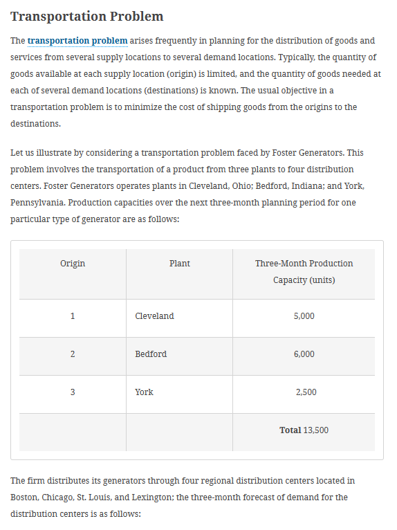
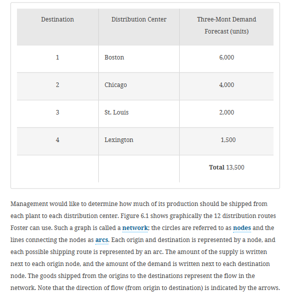
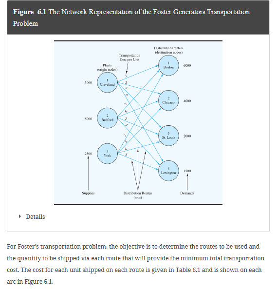
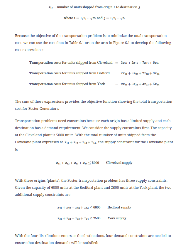
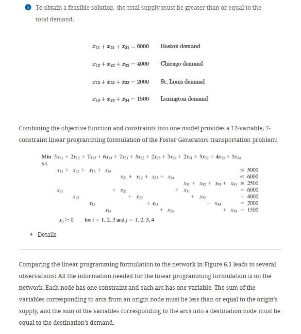
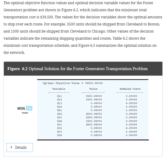
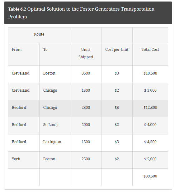
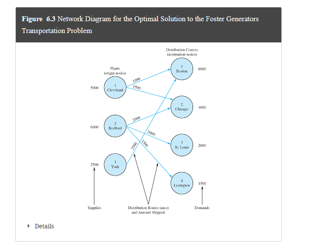
Table 6.2 Optimal Solution to the Foster Generators Transportation Problem Table 6.1 Transportation Cost per Unit for the Foster Generators Transportation Problem A linear programming model can be used to solve this transportation problem. We use doublesubscripted decision variables, with x11 denoting the number of units shipped from origin 1 (Cleveland) to destination 1 (Boston), x12 denoting the number of units shipped from origin 1 (Cleveland) to destination 2 (Chicago), and so on. In general, the decision variables for a transportation problem having m origins and n destinations are written as follows: Management would like to determine how much of its production should be shipped from each plant to each distribution center. Figure 6.1 shows graphically the 12 distribution routes Foster can use. Such a graph is called a network; the circles are referred to as nodes and the lines connecting the nodes as arcs. Each origin and destination is represented by a node, and each possible shipping route is represented by an arc. The amount of the supply is written next to each origin node, and the amount of the demand is written next to each destination node. The goods shipped from the origins to the destinations represent the flow in the network. Note that the direction of flow (from origin to destination) is indicated by the arrows. Transportation Problem The transportation problem arises frequently in planning for the distribution of goods and services from several supply locations to several demand locations. Typically, the quantity of goods available at each supply location (origin) is limited, and the quantity of goods needed at each of several demand locations (destinations) is known. The usual objective in a transportation problem is to minimize the cost of shipping goods from the origins to the destinations. Let us illustrate by considering a transportation problem faced by Foster Generators. This problem involves the transportation of a product from three plants to four distribution centers. Foster Generators operates plants in Cleveland, Ohio; Bedford, Indiana; and York, Pennsylvania. Production capacities over the next three-month planning period for one particular type of generator are as follows: The firm distributes its generators through four regional distribution centers located in Boston, Chicago, St. Louis, and Lexington; the three-month forecast of demand for the distribution centers is as follows: Figure 6.3 Network Diagram for the Optimal Solution to the Foster Generators Transportation Problem Details Figure 6.1 The Network Representation of the Foster Generators Transportation Problem Details For Foster's transportation problem, the objective is to determine the routes to be used and the quantity to be shipped via each route that will provide the minimum total transportation cost. The cost for each unit shipped on each route is given in Table 6.1 and is shown on each arc in Figure 6.1. xij=numberofunitsshippedfromoriginitodestinationj where i=1,2,,m and j=1,2,,n Because the objective of the transportation problem is to minimize the total transportation cost, we can use the cost data in Table 6.1 or on the arcs in Figure 6.1 to develop the following cost expressions: Transportation costs for units shipped from Cleveland =3x11+2x12+7x13+6x14 Transportation costs for units shipped from Bedford =7x21+5x22+2x23+3x24 Transportation costs for units shipped from York =2x31+5x32+4x33+5x34 The sum of these expressions provides the objective function showing the total transportation cost for Foster Generators. Transportation problems need constraints because each origin has a limited supply and each destination has a demand requirement. We consider the supply constraints first. The capacity at the Cleveland plant is 5000 units. With the total number of units shipped from the Cleveland plant expressed as x11+x12+x13+x14, the supply constraint for the Cleveland plant is x11+x12+x13+x145000Clevelandsupply With three origins (plants), the Foster transportation problem has three supply constraints. Given the capacity of 6000 units at the Bedford plant and 2500 units at the York plant, the two additional supply constraints are x21+x22+x23+x246000x31+x32+x33+x342500BedfordsupplyYorksupply With the four distribution centers as the destinations, four demand constraints are needed to ensure that destination demands will be satisfied: The optimal objective function values and optimal decision variable values for the Foster Generators problem are shown in Figure 6.2, which indicates that the minimum total transportation cost is $39,500. The values for the decision variables show the optimal amount to ship over each route. For example, 3500 units should be shipped from Cleveland to Boston, and 1500 units should be shipped from Cleveland to Chicago. Other values of the decision variables indicate the remaining shipping quantities and routes. Table 6.2 shows the minimum cost transportation schedule, and Figure 6.3 summarizes the optimal solution on the network. Figure 6.2 Optimal Solution for the Foster Generators Transportation Problem To obtain a feasible solution, the total supply must be greater than or equal to the total demand. x11+x21+x31=6000x12+x22+x32=4000x13+x23+x33=2000x14+x24+x34=1500BostondemandChicagodemandSt.LouisdemandLexingtondemand Combining the objective function and constraints into one model provides a 12-variable, 7constraint linear programming formulation of the Foster Generators transportation problem: Min3x11+2x12+7x13+6x14+7x21+5x22+2x23+3x24+2x31+5x32+4x33+5x34s.t.x11+x12+x13+x14x21+x22+x23+x24x11x31+x32+x33+x34+x212500=6000x12x13+x22+x3250006000=6000=4000=2000x14+x24+x33+x34=1500xij0fori=1,2,3andj=1,2,3,4 Details Comparing the linear programming formulation to the network in Figure 6.1 leads to several observations: All the information needed for the linear programming formulation is on the network. Each node has one constraint and each arc has one variable. The sum of the variables corresponding to arcs from an origin node must be less than or equal to the origin's supply, and the sum of the variables corresponding to the arcs into a destination node must be equal to the destination's demand. Table 6.2 Optimal Solution to the Foster Generators Transportation Problem Table 6.1 Transportation Cost per Unit for the Foster Generators Transportation Problem A linear programming model can be used to solve this transportation problem. We use doublesubscripted decision variables, with x11 denoting the number of units shipped from origin 1 (Cleveland) to destination 1 (Boston), x12 denoting the number of units shipped from origin 1 (Cleveland) to destination 2 (Chicago), and so on. In general, the decision variables for a transportation problem having m origins and n destinations are written as follows: Management would like to determine how much of its production should be shipped from each plant to each distribution center. Figure 6.1 shows graphically the 12 distribution routes Foster can use. Such a graph is called a network; the circles are referred to as nodes and the lines connecting the nodes as arcs. Each origin and destination is represented by a node, and each possible shipping route is represented by an arc. The amount of the supply is written next to each origin node, and the amount of the demand is written next to each destination node. The goods shipped from the origins to the destinations represent the flow in the network. Note that the direction of flow (from origin to destination) is indicated by the arrows. Transportation Problem The transportation problem arises frequently in planning for the distribution of goods and services from several supply locations to several demand locations. Typically, the quantity of goods available at each supply location (origin) is limited, and the quantity of goods needed at each of several demand locations (destinations) is known. The usual objective in a transportation problem is to minimize the cost of shipping goods from the origins to the destinations. Let us illustrate by considering a transportation problem faced by Foster Generators. This problem involves the transportation of a product from three plants to four distribution centers. Foster Generators operates plants in Cleveland, Ohio; Bedford, Indiana; and York, Pennsylvania. Production capacities over the next three-month planning period for one particular type of generator are as follows: The firm distributes its generators through four regional distribution centers located in Boston, Chicago, St. Louis, and Lexington; the three-month forecast of demand for the distribution centers is as follows: Figure 6.3 Network Diagram for the Optimal Solution to the Foster Generators Transportation Problem Details Figure 6.1 The Network Representation of the Foster Generators Transportation Problem Details For Foster's transportation problem, the objective is to determine the routes to be used and the quantity to be shipped via each route that will provide the minimum total transportation cost. The cost for each unit shipped on each route is given in Table 6.1 and is shown on each arc in Figure 6.1. xij=numberofunitsshippedfromoriginitodestinationj where i=1,2,,m and j=1,2,,n Because the objective of the transportation problem is to minimize the total transportation cost, we can use the cost data in Table 6.1 or on the arcs in Figure 6.1 to develop the following cost expressions: Transportation costs for units shipped from Cleveland =3x11+2x12+7x13+6x14 Transportation costs for units shipped from Bedford =7x21+5x22+2x23+3x24 Transportation costs for units shipped from York =2x31+5x32+4x33+5x34 The sum of these expressions provides the objective function showing the total transportation cost for Foster Generators. Transportation problems need constraints because each origin has a limited supply and each destination has a demand requirement. We consider the supply constraints first. The capacity at the Cleveland plant is 5000 units. With the total number of units shipped from the Cleveland plant expressed as x11+x12+x13+x14, the supply constraint for the Cleveland plant is x11+x12+x13+x145000Clevelandsupply With three origins (plants), the Foster transportation problem has three supply constraints. Given the capacity of 6000 units at the Bedford plant and 2500 units at the York plant, the two additional supply constraints are x21+x22+x23+x246000x31+x32+x33+x342500BedfordsupplyYorksupply With the four distribution centers as the destinations, four demand constraints are needed to ensure that destination demands will be satisfied: The optimal objective function values and optimal decision variable values for the Foster Generators problem are shown in Figure 6.2, which indicates that the minimum total transportation cost is $39,500. The values for the decision variables show the optimal amount to ship over each route. For example, 3500 units should be shipped from Cleveland to Boston, and 1500 units should be shipped from Cleveland to Chicago. Other values of the decision variables indicate the remaining shipping quantities and routes. Table 6.2 shows the minimum cost transportation schedule, and Figure 6.3 summarizes the optimal solution on the network. Figure 6.2 Optimal Solution for the Foster Generators Transportation Problem To obtain a feasible solution, the total supply must be greater than or equal to the total demand. x11+x21+x31=6000x12+x22+x32=4000x13+x23+x33=2000x14+x24+x34=1500BostondemandChicagodemandSt.LouisdemandLexingtondemand Combining the objective function and constraints into one model provides a 12-variable, 7constraint linear programming formulation of the Foster Generators transportation problem: Min3x11+2x12+7x13+6x14+7x21+5x22+2x23+3x24+2x31+5x32+4x33+5x34s.t.x11+x12+x13+x14x21+x22+x23+x24x11x31+x32+x33+x34+x212500=6000x12x13+x22+x3250006000=6000=4000=2000x14+x24+x33+x34=1500xij0fori=1,2,3andj=1,2,3,4 Details Comparing the linear programming formulation to the network in Figure 6.1 leads to several observations: All the information needed for the linear programming formulation is on the network. Each node has one constraint and each arc has one variable. The sum of the variables corresponding to arcs from an origin node must be less than or equal to the origin's supply, and the sum of the variables corresponding to the arcs into a destination node must be equal to the destination's demand