Assignment 1 README w2021.rtf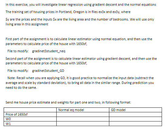

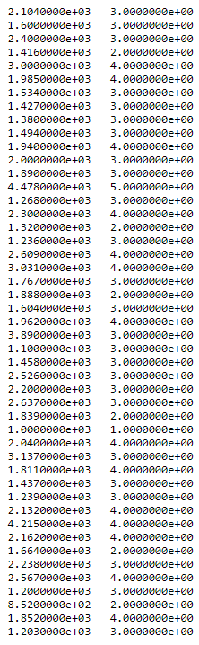
ex3x.dat:

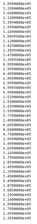
ex3y.dat :

gradient3 student GD.m :

gradient3student neq.m :

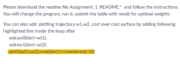
PLEASE help step by step with explanation for understanding.

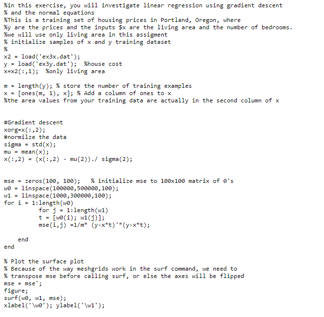
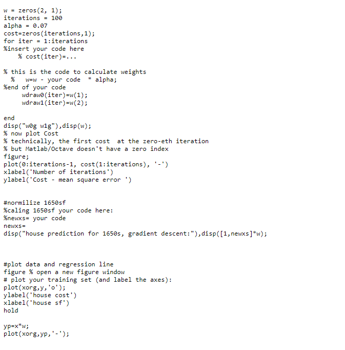
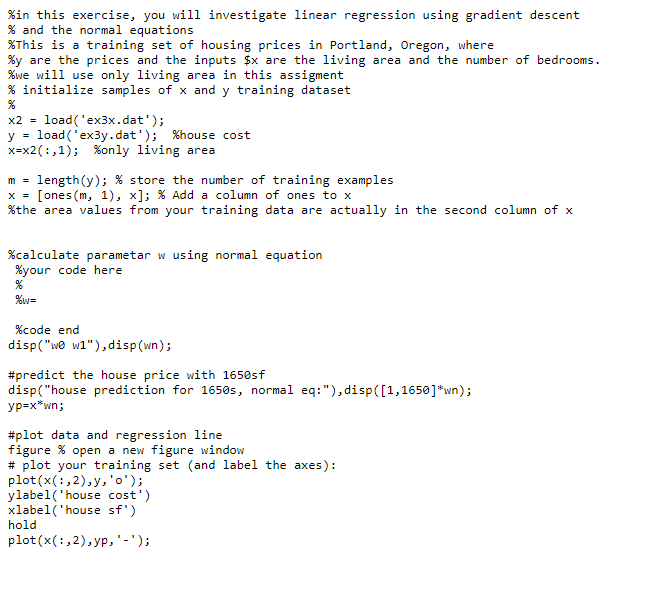
Please download the readme file Assignment_1_README.* and follow the instructions. You will change the program, run it, submit the table with result for optimal weights You can also add plotting trajectory w1,w2, cost over cost surface by adding following highlighted line inside the loop after wdrawO( iter )=w(1); wdraw 1( iter )=w(2) plot3(w(1),w(2),cost(iter),'rv",'markersize',10) The training set of housing prices in Portland, Oregon is in files ex3x and ex3y, where Sy are the prices and the inputs $x are the living area and the number of bedrooms. We will use only living area in this assignment First part of the assignment is to calculate linear estimator using normal equation, and then use the parameters to calculate price of the house with 1650 sf, File to modify: gradinet3student_neq Second part of the assignment is to calculate linear estimator using gradient descent, and then use the parameters to calculate price of the house with 1650 sf, File to modify: gradinet3student_GD Note: Recall when you are applying GD, it is good practice to normalize the input data (subtract the average and scale by standard deviation), to bring all data in the similar range. During prediction you need to do the same. Send me house price estimate and weights for part one and two, in following format: 2.1040000e+031.6000000e+032.4000000e+031.4160000e+033.0000000e+031.9850000e+031.5340000e+031.4270000e+031.3800000e+031.4940000e+031.9400000e+032.0000000e+031.8900000e+034.4780000e+031.2680000e+032.3000000e+031.3200000e+031.2360000e+032.6090000e+033.0310000e+031.7670000e+031.8880000e+031.6040000e+031.9620000e+033.8900000e+031.1000000e+031.4580000e+032.5260000e+032.2000000e+032.6370000e+031.8390000e+031.0000000e+032.0400000e+033.1370000e+031.8110000e+031.4370000e+031.520000000e+031.2030000e+033.0000000e+003.0000000e+003.0000000e+002.0000000e+004.0000000e+004.0000000e+003.0000000e+003.0000000e+003.0000000e+003.0000000e+004.0000000e+003.0000000e+003.0000000e+005.0000000e+003.0000000e+004.0000000e+002.0000000e+003.0000000e+004.0000000e+004.0000000e+003.0000000e+002.0000000e+003.0000000e+004.0000000e+003.0000000e+003.0000000e+003.0000000e+003.0000000e+003.0000000e+003.0000000e+002.0000000e+001.0000000e+004.0000000e+003.0000000e+004.0000000e+003.0000000e+003.0000000e+003.0000000e+00 3.9990000e+053.2990000e+053.6900000e+052.3200000e+055.3990000e+052.9990000e+053.1490000e+051.9899900e+052.1200000e+052.4250000e+052.3999900e+053.4700000e+053.2999900e+056.9990000e+052.5990000e+054.4990000e+052.9990000e+051.9990000e+054.9999800e+055.9900000e+052.5290000e+052.5500000e+052.4290000e+052.5990000e+055.7390000e+052.4990000e+054.6450000e+054.6900000e+054.7500000e+052.9990000e+053.4990000e+051.6990000e+053.1490000e+055.7990000e+052.8590000e+052.4990000e+052.2990000e+053.4500000e+055.4900000e+052.8700000e+053.6850000e+053.2990000e+053.1400000e+052.9900000e+051.7990000e+052.9990000e+052.3950000e+05 \%in this exercise, you will investigate linear regression using gradient descent % and the normal equations \%This is a training set of housing prices in Portland, Oregon, where \%y are the prices and the inputs $x are the living area and the number of bedrooms. \%we will use only living area in this assigment \% initialize samples of x and y training dataset % x2=load( 'ex 3xdat); y=load( 'ex3y.dat'); \%house cost x=x2(:,1); \%only living area m= length (y);% store the number of training examples x=[ ones (m,1),x]; Add a column of ones to x \%the area values from your training data are actually in the second column of x \%calculate parametar w using normal equation \%your code here % %w= \%code end disp("w0 w1"), disp(wn); \#predict the house price with 1650sf disp("house prediction for 16505 , normal eq:"), disp([1,1650]*wn); yp=xwn \#plot data and regression line figure % open a new figure window \# plot your training set (and label the axes): plot(x(:,2),y,0; ) ylabel ('house cost') xlabel ('house sf') hold plot(x(:,2),yp,)