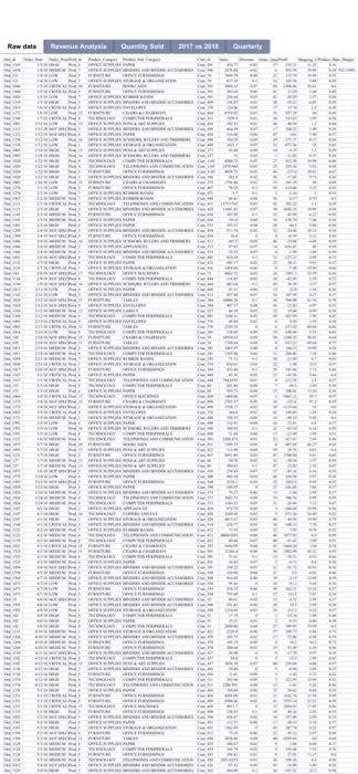
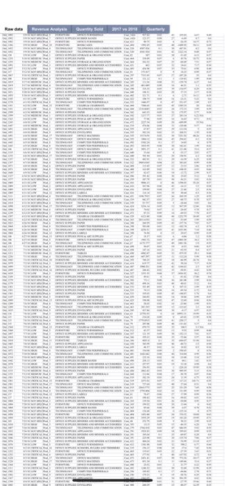
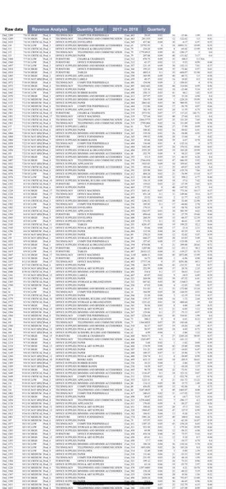
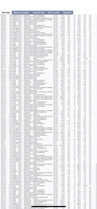
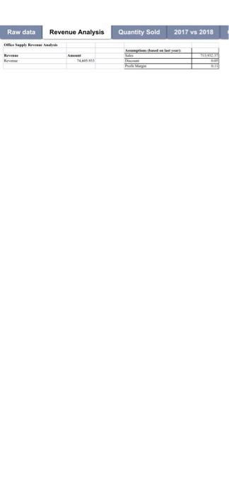
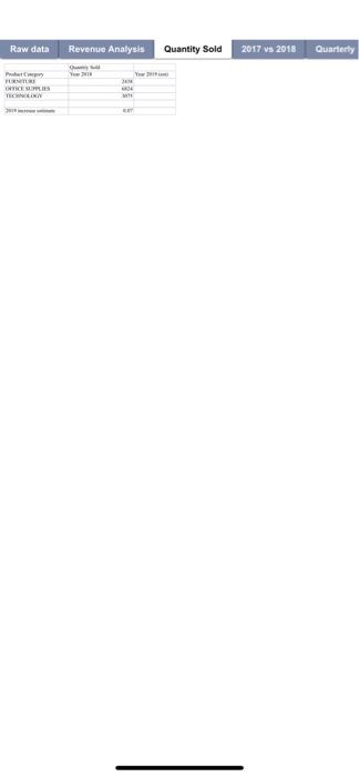
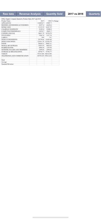
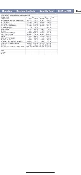
Assignment: Excel (75 points) Read the brief case below. Using the Excel spreadsheet provided, complete the questions. Downtown Office Supply Downtown Office supply is a small family owned store in a small suburb. In order to maintain and grow the business the owners want to do some analysis to see how their sales are doing, Management wants to see how the company did last year and make some decisions about what products to keep along with staffing for busy times of the year. Instructions: In the excle spreadheet provided, complete the tasks below. Upon completion you will submit a single completed, Excel workbook. 10 points each 1. Setup the spreadsheet with proper formatting and formulas so it can be presented to management. a. Change the tab called "Quarterly" to "QI - Quarterly" and move the tab to the first position. b. Add a column to calculate the total for each product. Use the SUM function. c. Add rows to calculate the Total, Average and Median sales for each quarter. Use the SUM, AVERAGE, and MEDIAN functions. d. Format the title at the top so it stands out. Add distinct formatting to the column and row headings. Format the data in the cells to show currency. e. Format the total sales column to have a green background. f. Create a bar chart showing for each product (a) the total sales for the year and (b) the proportion of the total contributed by each quarter's sales. This should be shown in one. You should have I bar for cach product. Add a title to your chart. 2. Management would like to decide whether they should discontinue any products. Any product which has had 50% less sales over the previous year should be discontinued. Are there any products that they should discontinued? List the product(s) and your recommendation in the worksheet. Which 3 products had the highest increase in sales? a. Change the tab called 2017 vs 2018 to Q2-2017 vs. 2018 and move the tab to the second position. b. Add a new column to calculate the percentage change from 2017 to 2018. Percentage change is computed using the following formula: (current year sales last year sales) / (last year sales). Represent the numbers as percentages. c. Calculate the total, average, and standard deviation for each year. d. Format the title at the top so it stands out. Add distinct formatting to the column and row headings. Format the data in the cells to show currency. e. Use conditional formatting to highlight the Percent Change cells that have a negative percent change in red. f. Use conditional formatting to highlight the top 3 cells that had the highest increase in green. g. Create a pie chart showing the contribution of each product to 2018 total sales. Make sure the percentages are displayed on the chart and the product names are displayed in the legend. Add a title to the chart. h. Which product was the highest contributor in 2018? (write the answer directly into the worksheet). 3. Management would to predict sales for next year using an increase estimate that they can change a. Change the tab called Quantity Sold to Q3 - Quantity Sold and move the tab to the third position. b. Compute the 2019 estimates for each group using the following formula: [2018 quantity sold + (2018 quantity sold the increase estimate)]. The increase estimate is shown in cell B7 c. Change the increase estimate to.10. The values should change automatically. When student create the formula they need to use an "absolute" reference: -B3+(B3 SBS) d. Format the title at the top so it stands out. Add distinct formatting to the column and row headings. Format the data in the cells to be whole numbers. e. Create a chart showing the distribution of quantity sold in 2018 for each product category. Add a title to the chart 4. Use the data in the sheet titled "Raw data" to calculate the profit for each product category and product sub category (ability to drill down) a. Create a new worksheet titled "Q4 - Profit by Category" and insert a new pivot table for the data in the sheet - "Raw Data". Move the worksheet to the 4 position. b. List the total profit for product categories and subcategories in this table c. Format the numbers to reflect the "S" symbol before the figures and 2 decimal places d. Change the column headines to be meaningful. c. Add a meaningful title to the worksheet at the top and center it across the pivot table. f. Use conditional bars to highlight gains and losses. g. Add another column to the pivot table display the profit or loss as a percent of the total. h. Use conditional formatting to display the top 3 products that had the highest percentage. 5. Management would like to know when their busiest month for sales is 1. Create a new worksheet titled "Q5-Sales by Month" and insert a new pivot table for the data in the sheet - "Raw Data". Move the worksheet after Q4 worksheet. b. List only the months in the 1 column and the sales in the 2 column. To do this click on one of the dates. Then do a right mouse click to display a menu. Click the Group option. Another menu will display. Click on Months and Quarters. c. Sort the sales in Descending order. d. Format the numbers to reflect the "S" symbol before the figures and 2 decimal places. c. Change the column heading to be meaningful f. Add a meaningful title to the worksheet at the top and center it across the pivot table. g. Use to conditional formatting to highlight the top month for sales in green, the bottom month for sales in red. h. Next, add a filter at the top so that you can filter out product sub categories 6. Management would like to know what is the split in terms of profit, across the Product Categories, for each quarter. Use a Line Chart to show the numbers. Rank the Product categories in terms of profit. a. Create a new worksheet titled-06 - Otr. Profit" and insert a new pivot table for the data in the sheet - "Raw data". Move the worksheet after Q3 worksheet. b. List all the Product Categories in the Ist column. c. Split the Quarter across the categories [ Hint: Drag the Date field in the "Column Label area). To group the date by Quarter - Click on the date field. Next, right mouse click to display a menu. Click the Group option. Another menu will display. Click on Months and Quarters d. Add the profit by category and quarter. Format the data in currency format Add manningful hal e. Add meaningful column labels. f. Add a meaningful title to the worksheet at the top and center it across the pivot table. g. Select the Pivot Table and Click on Options> Pivot Chart h. Insert a Column Chart of your choice. 7. One useful function of spreadsheet software is the ability to change input values and see the impact on outcome variables. For example, you can change sales projections and see the impact on net income. Excel's Scenario Manager makes performing these sorts of sensitivity analyses much easier. Goal-Seek Analysis Scenario Manager helps examine how changes in input values impact outcome variables. To perform this analysis, go to the Data ribbon and select What If Analysis, then Goal- Seek. a. Change the title of worksheet "Revenue Analysis" to "Q7 - Revenue Analysis" and move it after Q6 worksheet b. Answer the following questions directly into the worksheet: i. What do sales need to be in order to reach 100,000 in revenue? ii. What does the profit margin need to be to reach 100,000 in revenue? 5 points 8. Prepare your analysis for Management. Create a Table of Contents a. Create a new worksheet and move it to the beginning, This worksheet should list the contents of the workbook along with the purpose of the workbook. the current date and the name of the person who created the workbook. Be sure to have titles for each of these b. Make cach list item a hyperlink to that particular workbook. For example, in the table of contents you will have an item titled "QI - Quarterly Sales". Create a hyperlink to link to that particular workbook. c. Move the Raw Data to the last position d. User proper elements to add the file name and current date to the header Raw data Mave Any Quantity Sed 2017 2018 Cure Raw data Sea 2017 2018 Quran SEITE! - THE FELIS BREVET FREE FRETERETETTEL Raw date Quantity Set 2017 2018 Our bisik.clic TETTIIEEE 15155 BE115 Raw data Marvenue Analyse Quantity Sord 2017 2018 Guara tiitti REKTE Quantity Sold 2017 vs 2018 Raw data Revenue Analysis e Sepp Headh RAM Rem waar D. Raw data Revenue Analysis Quantity Sold 2017 vs 2018 Quarterly RICES Raw data Revenue Analysis Quantity Sold 2017 vs 2018 Quarterly ALLANES NDERS AND INTERVISTA BURAS CURS & CRMATS CORALS COPERSANDIAN INS LARIS WERONI ONE MACHINES HARTS TRANS SCIOUS RESOS RADATION TABLES TELES DE UMAT Total w 14 9045 w Raw data Revenue Analysis Quantity Sold 2017 vs 2018 Qual O Supply Co Oy Pro 01 GC APPLIANCES SENDERSANES BINDER MCESSORIES 1126 BOOKCASES TH CHAIRS CHAIRMAN 40 CHAPTERIALS COPIES ANTAN INVELOPES LARES OLICE FURNISHINOS 1433 13 DE MACHINES 0411 PAPER TAMAN PENSATSEN BURADA 3 TSONS, NUR NOTRES SOMOS A CALZATUN 18 CARLES 10 MORT TELEPHONES AND COMMUNICATIONSWE Assignment: Excel (75 points) Read the brief case below. Using the Excel spreadsheet provided, complete the questions. Downtown Office Supply Downtown Office supply is a small family owned store in a small suburb. In order to maintain and grow the business the owners want to do some analysis to see how their sales are doing, Management wants to see how the company did last year and make some decisions about what products to keep along with staffing for busy times of the year. Instructions: In the excle spreadheet provided, complete the tasks below. Upon completion you will submit a single completed, Excel workbook. 10 points each 1. Setup the spreadsheet with proper formatting and formulas so it can be presented to management. a. Change the tab called "Quarterly" to "QI - Quarterly" and move the tab to the first position. b. Add a column to calculate the total for each product. Use the SUM function. c. Add rows to calculate the Total, Average and Median sales for each quarter. Use the SUM, AVERAGE, and MEDIAN functions. d. Format the title at the top so it stands out. Add distinct formatting to the column and row headings. Format the data in the cells to show currency. e. Format the total sales column to have a green background. f. Create a bar chart showing for each product (a) the total sales for the year and (b) the proportion of the total contributed by each quarter's sales. This should be shown in one. You should have I bar for cach product. Add a title to your chart. 2. Management would like to decide whether they should discontinue any products. Any product which has had 50% less sales over the previous year should be discontinued. Are there any products that they should discontinued? List the product(s) and your recommendation in the worksheet. Which 3 products had the highest increase in sales? a. Change the tab called 2017 vs 2018 to Q2-2017 vs. 2018 and move the tab to the second position. b. Add a new column to calculate the percentage change from 2017 to 2018. Percentage change is computed using the following formula: (current year sales last year sales) / (last year sales). Represent the numbers as percentages. c. Calculate the total, average, and standard deviation for each year. d. Format the title at the top so it stands out. Add distinct formatting to the column and row headings. Format the data in the cells to show currency. e. Use conditional formatting to highlight the Percent Change cells that have a negative percent change in red. f. Use conditional formatting to highlight the top 3 cells that had the highest increase in green. g. Create a pie chart showing the contribution of each product to 2018 total sales. Make sure the percentages are displayed on the chart and the product names are displayed in the legend. Add a title to the chart. h. Which product was the highest contributor in 2018? (write the answer directly into the worksheet). 3. Management would to predict sales for next year using an increase estimate that they can change a. Change the tab called Quantity Sold to Q3 - Quantity Sold and move the tab to the third position. b. Compute the 2019 estimates for each group using the following formula: [2018 quantity sold + (2018 quantity sold the increase estimate)]. The increase estimate is shown in cell B7 c. Change the increase estimate to.10. The values should change automatically. When student create the formula they need to use an "absolute" reference: -B3+(B3 SBS) d. Format the title at the top so it stands out. Add distinct formatting to the column and row headings. Format the data in the cells to be whole numbers. e. Create a chart showing the distribution of quantity sold in 2018 for each product category. Add a title to the chart 4. Use the data in the sheet titled "Raw data" to calculate the profit for each product category and product sub category (ability to drill down) a. Create a new worksheet titled "Q4 - Profit by Category" and insert a new pivot table for the data in the sheet - "Raw Data". Move the worksheet to the 4 position. b. List the total profit for product categories and subcategories in this table c. Format the numbers to reflect the "S" symbol before the figures and 2 decimal places d. Change the column headines to be meaningful. c. Add a meaningful title to the worksheet at the top and center it across the pivot table. f. Use conditional bars to highlight gains and losses. g. Add another column to the pivot table display the profit or loss as a percent of the total. h. Use conditional formatting to display the top 3 products that had the highest percentage. 5. Management would like to know when their busiest month for sales is 1. Create a new worksheet titled "Q5-Sales by Month" and insert a new pivot table for the data in the sheet - "Raw Data". Move the worksheet after Q4 worksheet. b. List only the months in the 1 column and the sales in the 2 column. To do this click on one of the dates. Then do a right mouse click to display a menu. Click the Group option. Another menu will display. Click on Months and Quarters. c. Sort the sales in Descending order. d. Format the numbers to reflect the "S" symbol before the figures and 2 decimal places. c. Change the column heading to be meaningful f. Add a meaningful title to the worksheet at the top and center it across the pivot table. g. Use to conditional formatting to highlight the top month for sales in green, the bottom month for sales in red. h. Next, add a filter at the top so that you can filter out product sub categories 6. Management would like to know what is the split in terms of profit, across the Product Categories, for each quarter. Use a Line Chart to show the numbers. Rank the Product categories in terms of profit. a. Create a new worksheet titled-06 - Otr. Profit" and insert a new pivot table for the data in the sheet - "Raw data". Move the worksheet after Q3 worksheet. b. List all the Product Categories in the Ist column. c. Split the Quarter across the categories [ Hint: Drag the Date field in the "Column Label area). To group the date by Quarter - Click on the date field. Next, right mouse click to display a menu. Click the Group option. Another menu will display. Click on Months and Quarters d. Add the profit by category and quarter. Format the data in currency format Add manningful hal e. Add meaningful column labels. f. Add a meaningful title to the worksheet at the top and center it across the pivot table. g. Select the Pivot Table and Click on Options> Pivot Chart h. Insert a Column Chart of your choice. 7. One useful function of spreadsheet software is the ability to change input values and see the impact on outcome variables. For example, you can change sales projections and see the impact on net income. Excel's Scenario Manager makes performing these sorts of sensitivity analyses much easier. Goal-Seek Analysis Scenario Manager helps examine how changes in input values impact outcome variables. To perform this analysis, go to the Data ribbon and select What If Analysis, then Goal- Seek. a. Change the title of worksheet "Revenue Analysis" to "Q7 - Revenue Analysis" and move it after Q6 worksheet b. Answer the following questions directly into the worksheet: i. What do sales need to be in order to reach 100,000 in revenue? ii. What does the profit margin need to be to reach 100,000 in revenue? 5 points 8. Prepare your analysis for Management. Create a Table of Contents a. Create a new worksheet and move it to the beginning, This worksheet should list the contents of the workbook along with the purpose of the workbook. the current date and the name of the person who created the workbook. Be sure to have titles for each of these b. Make cach list item a hyperlink to that particular workbook. For example, in the table of contents you will have an item titled "QI - Quarterly Sales". Create a hyperlink to link to that particular workbook. c. Move the Raw Data to the last position d. User proper elements to add the file name and current date to the header Raw data Mave Any Quantity Sed 2017 2018 Cure Raw data Sea 2017 2018 Quran SEITE! - THE FELIS BREVET FREE FRETERETETTEL Raw date Quantity Set 2017 2018 Our bisik.clic TETTIIEEE 15155 BE115 Raw data Marvenue Analyse Quantity Sord 2017 2018 Guara tiitti REKTE Quantity Sold 2017 vs 2018 Raw data Revenue Analysis e Sepp Headh RAM Rem waar D. Raw data Revenue Analysis Quantity Sold 2017 vs 2018 Quarterly RICES Raw data Revenue Analysis Quantity Sold 2017 vs 2018 Quarterly ALLANES NDERS AND INTERVISTA BURAS CURS & CRMATS CORALS COPERSANDIAN INS LARIS WERONI ONE MACHINES HARTS TRANS SCIOUS RESOS RADATION TABLES TELES DE UMAT Total w 14 9045 w Raw data Revenue Analysis Quantity Sold 2017 vs 2018 Qual O Supply Co Oy Pro 01 GC APPLIANCES SENDERSANES BINDER MCESSORIES 1126 BOOKCASES TH CHAIRS CHAIRMAN 40 CHAPTERIALS COPIES ANTAN INVELOPES LARES OLICE FURNISHINOS 1433 13 DE MACHINES 0411 PAPER TAMAN PENSATSEN BURADA 3 TSONS, NUR NOTRES SOMOS A CALZATUN 18 CARLES 10 MORT TELEPHONES AND COMMUNICATIONSWE