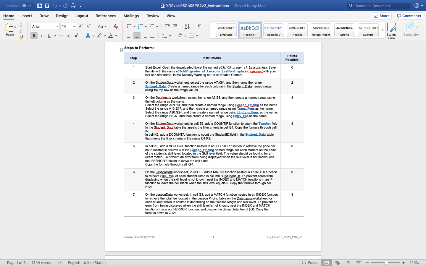
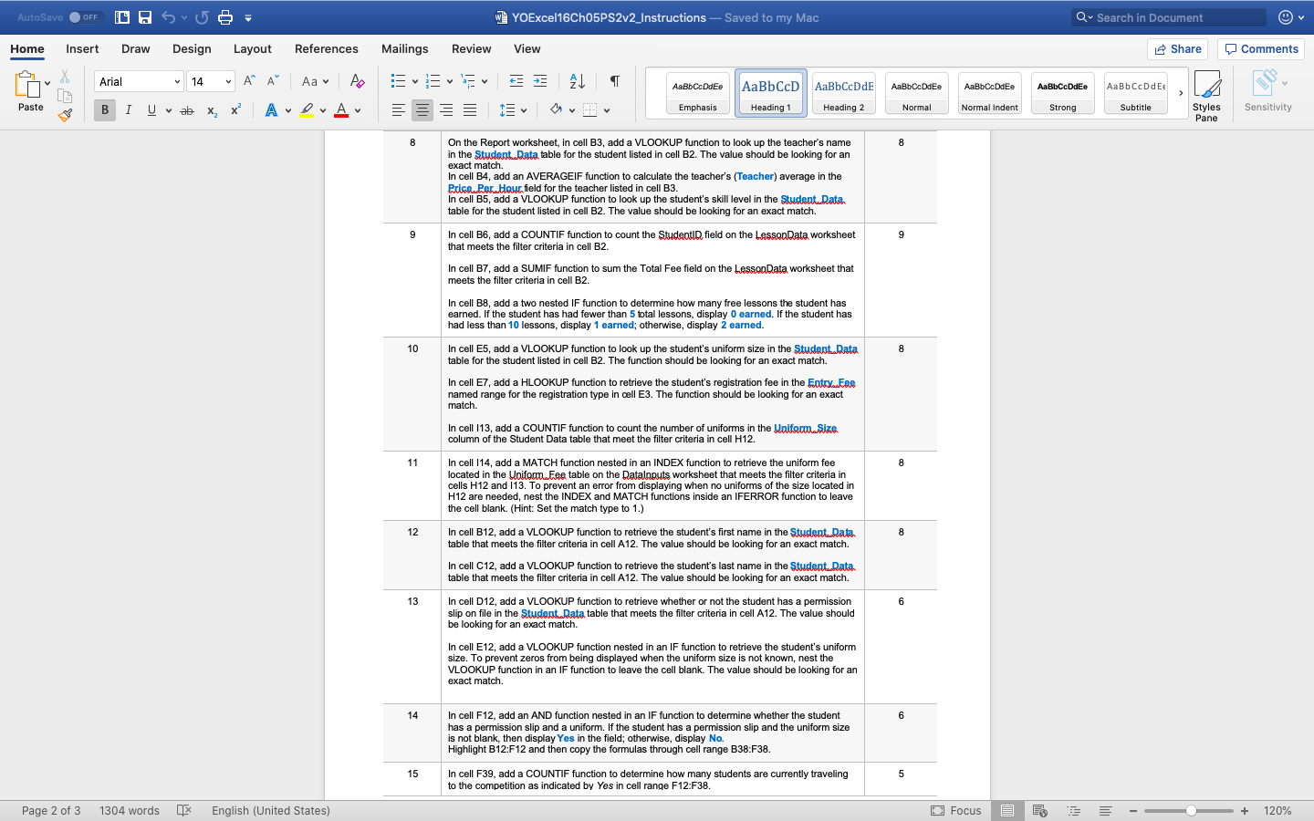
AutoSave OFF G Sv e : W YOExcel16Ch05PS2v2_Instructions - Saved to my Mac Q Search in Document Home Insert Draw Design Layout References Mailings Review View Comments Share Aabbccdder v Evv at AaBbcDdEe AaBbCcD AaBbCcDdE AaBbDdEe AaBbDcDdEe AaBbCcDdEe AaBBC DIE par Arial 14 V AC Aav Ao B IU ab X, X? ADA AaBbDcDdE+ Paste O Emphasis Heading 1 Heading 2 Normal Normal Indent Strong Subtitle Styles Pane Sensitivity + Steps to Perform: Step Instructions Points Possible Start Excel. Open the downloaded Excel file named e03ch05 grader a1 Lessons.xlsx. Save the file with the name e03ch05_grader_a1_Lessons LastFirst replacing LastFirst with your last and first name. In the Security Warning bar, click Enable Content. On the Student Data worksheet, select the range A7:K94, and then name the range Student Data, Create a named range for each column in the Student. Data named range, using the top row as the range values. On the Datalnputs worksheet, select the range A3:B3, and then create a named range using the left column as the name. Select the range A6:E10, and then create a named range using Lesson Pricing as the name. Select the range A13:E17, and then create a named range using Trans Fees, as the name. Select the range A20:G24, and then create a named range using Uniform Fees, as the name. Select the range H6J7, and then create a named range using Entry Fae as the name. 8 On the StudentData worksheet, in cell E5, add a COUNTIF function to count the Teacher field in the Student Data table that meets the filter criteria in cell E4. Copy the formula through cell In cell K5, add a DCOUNTA function to count the Studentin field in the Student Rata table that meets the filter criteria in the range D1:52. In cell KB, add a VLOOKUP function nested in an IFERROR function to retrieve the price per hour, located in column 3 in the Lesson Pricing named range, for each student on the basis of the student's skill level, located in the Skill level field. The value should be looking for an exact match. To prevent an error from being displayed when the skill level is not known, use the IFERROR function to leave the cell blank. Copy the formula through cell K94. 8 On the LessonData worksheet, in cell F3, add a MATCH function nested in an INDEX function to retrieve Skill level of each student listed in column B (StudentID). To prevent zeros from displaying when the skill level is not known, nest the INDEX and MATCH functions in an IF function to leave the cell blank when the skill level equals 0. Copy the formula through cell F121. 8 On the Lesson Data worksheet, in cell G3, add a MATCH function nested in an INDEX function to retrieve the total fee located in the Lesson Pricing table on the Dataloouts, worksheet for each student listed in column B depending on their lesson length and skill level. To prevent an error from being displayed when the skill level is not known, nest the INDEX and MATCH functions inside an IFERROR function, and display the default total fee of $50. Copy the formula down to G121. Created On: 07/05/2019 YO_Excel16_Ch05_PS2_V2 Page 1 of 3 1304 words English (United States) O Focus - + 120% AutoSave OFF G Sv e : W YOExcel16Ch05PS2v2_Instructions - Saved to my Mac Q Search in Document Home Insert Draw Design Layout References Mailings Review View Share Comments v Evv AaBbCcDdEe AaBb CcD AaBbCcDdE AaBbD:DaEe AaBbDcDdEe AaBbCcDdEe AaBbDcDdE+ par Arial 14 V AC Aav Ao B IU ab X, X? ADA Paste O Emphasis Heading 1 Heading 2 Normal Normal Indent Strong Subtitle Styles Pane Sensitivity On the Report worksheet, in cell B3, add a VLOOKUP function to look up the teacher's name in the Student Data table for the student listed in cell B2. The value should be looking for an exact match. In cell B4, add an AVERAGEIF function to calculate the teacher's (Teacher) average in the Price Per Hour field for the teacher listed in cell B3. In cell B5, add a VLOOKUP function to look up the student's skill level in the Student. Data table for the student listed in cell B2. The value should be looking for an exact match. In cell B6, add a COUNTIF function to count the Studentin field on the Lesson Data worksheet that meets the filter criteria in cell B2. In cell B7, add a SUMIF function to sum the Total Fee field on the Lesson Data worksheet that meets the filter criteria in cell B2. In cell B8, add a two nested IF function to determine how many free lessons the student has earned. If the student has had fewer than 5 total lessons, display O earned. If the student has had less than 10 lessons, display 1 earned; otherwise, display 2 earned. In cell E5, add a VLOOKUP function to look up the student's uniform size in the Student Data table for the student listed in cell B2. The function should be looking for an exact match. In cell E7, add a HLOOKUP function to retrieve the student's registration fee in the Entry Fee named range for the registration type in cell E3. The function should be looking for an exact match. In cell 113, add a COUNTIF function to count the number of uniforms in the Uniform...Size. column of the Student Data table that meet the filter criteria in cell H12. In cell 114, add a MATCH function nested in an INDEX function to retrieve the uniform fee located in the Uniform Fee table on the Datalnputs worksheet that meets the filter criteria in cells H12 and 113. To prevent an error from displaying when no uniforms of the size located in H12 are needed, nest the INDEX and MATCH functions inside an IFERROR function to leave the cell blank. (Hint: Set the match type to 1.) In cell B12, add a VLOOKUP function to retrieve the student's first name in the Student Rata. table that meets the filter criteria in cell A12. The value should be looking for an exact match. In cell C12, add a VLOOKUP function to retrieve the student's last name in the Student Data table that meets the filter criteria in cell A12. The value should be looking for an exact match. 6 In cell D12, add a VLOOKUP function to retrieve whether or not the student has a permission slip on file in the Student Data table that meets the filter criteria in cell A12. The value should be looking for an exact match. In cell E12, add a VLOOKUP function nested in an IF function to retrieve the student's uniform size. To prevent zeros from being displayed when the uniform size is not known, nest the VLOOKUP function in an IF function to leave the cell blank. The value should be looking for an exact match. 14 In cell F12, add an AND function nested in an IF function to determine whether the student has a permission slip and a uniform. If the student has a permission slip and the uniform size is not blank, then display Yes in the field; otherwise, display No. Highlight B12:F12 and then copy the formulas through cell range B38:F38. 15 In cell F39. add a COUNTIF function to determine how many students are currently traveling to the competition as indicated by Yes in cell range F12:F38. Page 2 of 3 1304 words English (United States) O Focus - + 120% AutoSave OFF G Sv e : W YOExcel16Ch05PS2v2_Instructions - Saved to my Mac Q Search in Document Home Insert Draw Design Layout References Mailings Review View Comments Share Aabbccdder v Evv at AaBbcDdEe AaBbCcD AaBbCcDdE AaBbDdEe AaBbDcDdEe AaBbCcDdEe AaBBC DIE par Arial 14 V AC Aav Ao B IU ab X, X? ADA AaBbDcDdE+ Paste O Emphasis Heading 1 Heading 2 Normal Normal Indent Strong Subtitle Styles Pane Sensitivity + Steps to Perform: Step Instructions Points Possible Start Excel. Open the downloaded Excel file named e03ch05 grader a1 Lessons.xlsx. Save the file with the name e03ch05_grader_a1_Lessons LastFirst replacing LastFirst with your last and first name. In the Security Warning bar, click Enable Content. On the Student Data worksheet, select the range A7:K94, and then name the range Student Data, Create a named range for each column in the Student. Data named range, using the top row as the range values. On the Datalnputs worksheet, select the range A3:B3, and then create a named range using the left column as the name. Select the range A6:E10, and then create a named range using Lesson Pricing as the name. Select the range A13:E17, and then create a named range using Trans Fees, as the name. Select the range A20:G24, and then create a named range using Uniform Fees, as the name. Select the range H6J7, and then create a named range using Entry Fae as the name. 8 On the StudentData worksheet, in cell E5, add a COUNTIF function to count the Teacher field in the Student Data table that meets the filter criteria in cell E4. Copy the formula through cell In cell K5, add a DCOUNTA function to count the Studentin field in the Student Rata table that meets the filter criteria in the range D1:52. In cell KB, add a VLOOKUP function nested in an IFERROR function to retrieve the price per hour, located in column 3 in the Lesson Pricing named range, for each student on the basis of the student's skill level, located in the Skill level field. The value should be looking for an exact match. To prevent an error from being displayed when the skill level is not known, use the IFERROR function to leave the cell blank. Copy the formula through cell K94. 8 On the LessonData worksheet, in cell F3, add a MATCH function nested in an INDEX function to retrieve Skill level of each student listed in column B (StudentID). To prevent zeros from displaying when the skill level is not known, nest the INDEX and MATCH functions in an IF function to leave the cell blank when the skill level equals 0. Copy the formula through cell F121. 8 On the Lesson Data worksheet, in cell G3, add a MATCH function nested in an INDEX function to retrieve the total fee located in the Lesson Pricing table on the Dataloouts, worksheet for each student listed in column B depending on their lesson length and skill level. To prevent an error from being displayed when the skill level is not known, nest the INDEX and MATCH functions inside an IFERROR function, and display the default total fee of $50. Copy the formula down to G121. Created On: 07/05/2019 YO_Excel16_Ch05_PS2_V2 Page 1 of 3 1304 words English (United States) O Focus - + 120% AutoSave OFF G Sv e : W YOExcel16Ch05PS2v2_Instructions - Saved to my Mac Q Search in Document Home Insert Draw Design Layout References Mailings Review View Share Comments v Evv AaBbCcDdEe AaBb CcD AaBbCcDdE AaBbD:DaEe AaBbDcDdEe AaBbCcDdEe AaBbDcDdE+ par Arial 14 V AC Aav Ao B IU ab X, X? ADA Paste O Emphasis Heading 1 Heading 2 Normal Normal Indent Strong Subtitle Styles Pane Sensitivity On the Report worksheet, in cell B3, add a VLOOKUP function to look up the teacher's name in the Student Data table for the student listed in cell B2. The value should be looking for an exact match. In cell B4, add an AVERAGEIF function to calculate the teacher's (Teacher) average in the Price Per Hour field for the teacher listed in cell B3. In cell B5, add a VLOOKUP function to look up the student's skill level in the Student. Data table for the student listed in cell B2. The value should be looking for an exact match. In cell B6, add a COUNTIF function to count the Studentin field on the Lesson Data worksheet that meets the filter criteria in cell B2. In cell B7, add a SUMIF function to sum the Total Fee field on the Lesson Data worksheet that meets the filter criteria in cell B2. In cell B8, add a two nested IF function to determine how many free lessons the student has earned. If the student has had fewer than 5 total lessons, display O earned. If the student has had less than 10 lessons, display 1 earned; otherwise, display 2 earned. In cell E5, add a VLOOKUP function to look up the student's uniform size in the Student Data table for the student listed in cell B2. The function should be looking for an exact match. In cell E7, add a HLOOKUP function to retrieve the student's registration fee in the Entry Fee named range for the registration type in cell E3. The function should be looking for an exact match. In cell 113, add a COUNTIF function to count the number of uniforms in the Uniform...Size. column of the Student Data table that meet the filter criteria in cell H12. In cell 114, add a MATCH function nested in an INDEX function to retrieve the uniform fee located in the Uniform Fee table on the Datalnputs worksheet that meets the filter criteria in cells H12 and 113. To prevent an error from displaying when no uniforms of the size located in H12 are needed, nest the INDEX and MATCH functions inside an IFERROR function to leave the cell blank. (Hint: Set the match type to 1.) In cell B12, add a VLOOKUP function to retrieve the student's first name in the Student Rata. table that meets the filter criteria in cell A12. The value should be looking for an exact match. In cell C12, add a VLOOKUP function to retrieve the student's last name in the Student Data table that meets the filter criteria in cell A12. The value should be looking for an exact match. 6 In cell D12, add a VLOOKUP function to retrieve whether or not the student has a permission slip on file in the Student Data table that meets the filter criteria in cell A12. The value should be looking for an exact match. In cell E12, add a VLOOKUP function nested in an IF function to retrieve the student's uniform size. To prevent zeros from being displayed when the uniform size is not known, nest the VLOOKUP function in an IF function to leave the cell blank. The value should be looking for an exact match. 14 In cell F12, add an AND function nested in an IF function to determine whether the student has a permission slip and a uniform. If the student has a permission slip and the uniform size is not blank, then display Yes in the field; otherwise, display No. Highlight B12:F12 and then copy the formulas through cell range B38:F38. 15 In cell F39. add a COUNTIF function to determine how many students are currently traveling to the competition as indicated by Yes in cell range F12:F38. Page 2 of 3 1304 words English (United States) O Focus - + 120%