b$.$ Correct the function used in cell A$3$ to calculate the sum of the values

in the NumAttending column.

c$.$ D$.$ Correct the function used in cell A$4$ to count the number of values in

the street column.

d$.7$ Correct the function used in cell $A5$ to count the number of blank cells

in the NumAttending column.

e$.$ Correct the function used in cell A$6$ to display the largest value in the

NumbAttending column

f$.$ Correct the function used in cell A$7$ to display the average value in the

NumAttending column

On the Shopping List sheet, check all the formulas. Cells to check are filled

with the light purple color. Most of them need to be corrected. Many of the

problems on this worksheet can be solved by creating named ranges or

using $f$ name that already exists.

$?$

a$.$ The formula in cell $B2$ uses the wrong function.

b$.$ The formulas in cells A$9$:A$23$ reference a named range that doesn't

exist. There is more than one correct way to fix this problem using the cell

range A$2$:H$15$ on the Places to Shop worksheet. You can create the named

range referenced in the formulas, or you can change the function

arguments to reference the cell range instead.

c$.$ The formula in cell $H99$ results in the correct value. However, the

workbook author copied this formula to the remaining cells in the column

and those values are definitely not correct! Fix the formula in cell H$9$ and

copy it to cells H$10$:H$23.$ Hint. Notice that cell H$8$ is named Tax.

If you've fixed the formulas in cells $H9$:$H23$ correctly, the formulas in cells

$19$:$123$ and G$5$ should calculate properly now. However, the formulas in cells

G$2$:G$4$ still have errors that need to be fixed. Hint: Use error checking as

needed and$/$or display the formulas on$-$screen for easy viewing.

a$.$ Correct the function used in cell $G2$ to average value of the Cost

column.

b$.$ Correct the function used in cell G$3$ to display the largest value in the

Cost column.

c$.$ Correct the function used in cell G$4$ to display the smallest value in the

Cost column.

On the Summary sheet, you will be entering all the formulas. Cells to

complete are filled with the light purple color. Hint: Use error checking as

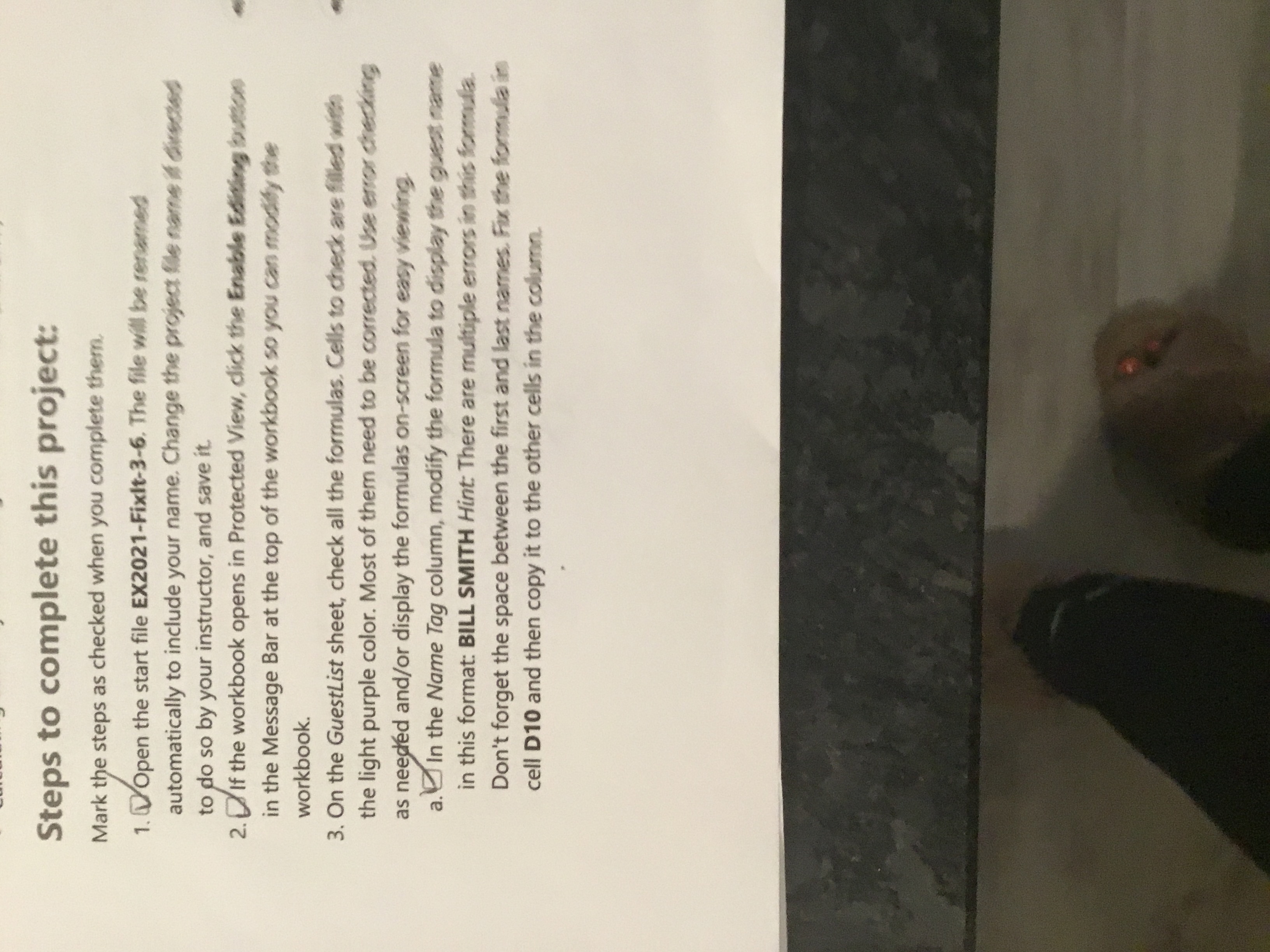
needed and$/$or display the formulas on$-$screen for easy viewing.Steps to complete this project:

Mark the steps as checked when you complete them.

Open the start file EX$2021-$FixIt$-3-6.$ The file will be renamed

automatically to include your name. Change the project ite name if divsetes

to do so by your instructor, and save it$.$

If the workbook opens in Protected View, click the Enable Edining button

in the Message Bar at the top of the workbook so you can modify the

workbook.

On the GuestList sheet, check all the formulas. Cells to check are filled with

the light purple color. Most of them need to be corrected. Use error checking

as neeged and$/$or display the formulas on$-$screen for easy viewing.

a$.$ In the Name Tag column, modify the formula to display the guest name

in this format: BILL SMITH Hint: There are multiple errors in this formula.

Don't forget the space between the first and last names. Fix the formula in

cell D$10$ and then copy it to the other cells in the column.