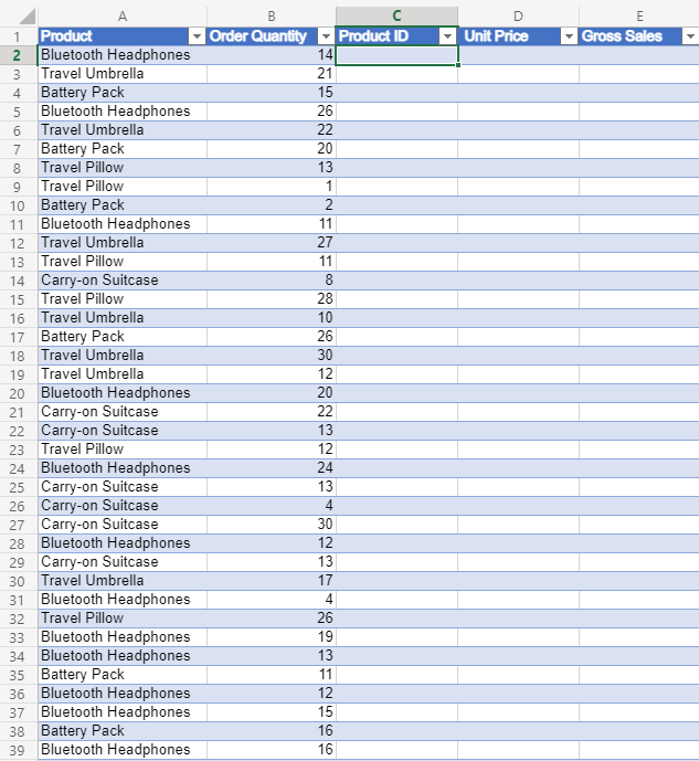
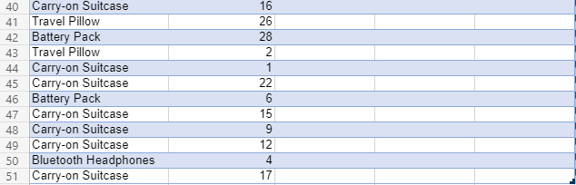
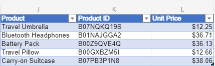
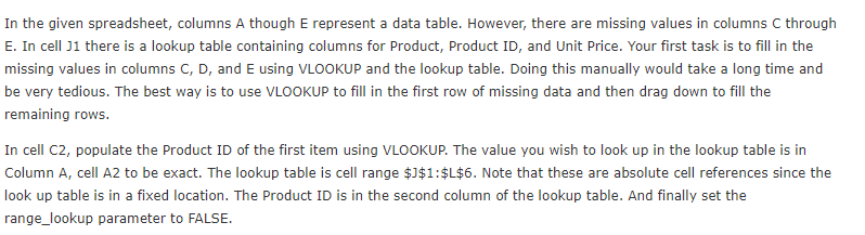
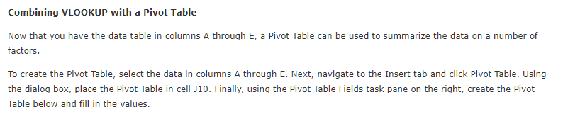
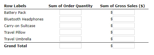
B D E Order Quantity Unit Price Gross Sales Ninco Product ID 14 21 15 26 22 20 13 1 Product 2 Bluetooth Headphones 3 Travel Umbrella 4 Battery Pack 5 Bluetooth Headphones 6 Travel Umbrella 7 Battery Pack 8 Travel Pillow 9 Travel Pillow 10 Battery Pack 11 Bluetooth Headphones 12 Travel Umbrella 13 Travel Pillow 14 Carry-on Suitcase 15 Travel Pillow 16 Travel Umbrella 17 Battery Pack 18 Travel Umbrella 19 Travel Umbrella 20 Bluetooth Headphones 21 Carry-on Suitcase 22 Carry-on Suitcase 23 Travel Pillow 24 Bluetooth Headphones 25 Carry-on Suitcase 26 Carry-on Suitcase 27 Carry-on Suitcase 28 Bluetooth Headphones 29 Carry-on Suitcase 30 Travel Umbrella 31 Bluetooth Headphones 32 Travel Pillow 33 Bluetooth Headphones 34 Bluetooth Headphones 35 Battery Pack 36 Bluetooth Headphones 37 Bluetooth Headphones 38 Battery Pack 39 Bluetooth Headphones 2 11 27 11 8 28 10 26 30 12 20 22 13 12 24 13 4 30 12 13 17 4 26 19 13 11 12 15 16 16 40 Carry-on Suitcase 41 Travel Pillow 42 Battery Pack 43 Travel Pillow 44 Carry-on Suitcase 45 Carry-on Suitcase 46 Battery Pack 47 Carry-on Suitcase 48 Carry-on Suitcase 49 Carry-on Suitcase 50 Bluetooth Headphones 51 Carry-on Suitcase 16 26 28 2 1 22 6 15 9 12 4 17 L Unit Price K Product Product ID Travel Umbrella BO7NQKQ195 Bluetooth Headphones B01NAJGGA2 Battery Pack BOOZ9QVE4Q Travel Pillow BOOGXBZM51 Carry-on Suitcase B07PB3P1N8 $12.25 $36.71 $36.13 $12.66 $38.06 In the given spreadsheet, columns A though E represent a data table. However, there are missing values in columns C through E. In cell J1 there is a lookup table containing columns for Product, Product ID, and Unit Price. Your first task is to fill in the missing values in columns C, D, and E using VLOOKUP and the lookup table. Doing this manually would take a long time and be very tedious. The best way is to use VLOOKUP to fill in the first row of missing data and then drag down to fill the remaining rows. In cell C2, populate the Product ID of the first item using VLOOKUP. The value you wish to look up in the lookup table is in Column A, cell A2 to be exact. The lookup table is cell range $J$1:$L$6. Note that these are absolute cell references since the look up table is in a fixed location. The Product ID is in the second column of the lookup table. And finally set the range_lookup parameter to FALSE. What is the Product ID returned in cell C2? Now repeat this process for the missing Unit Price in cell D2. What is the unit price returned in D2 (to the nearest cent)? And finally, for the first item, calculate the Gross Sales in column E using Order Quantity from column B and Unit Price from Column D. What is the gross sale amount in cell E2? To complete the data table, select cells C2, D2, and E2 together then drag down or double-click the fill + sign in the lower right of those three selected cells. And there you have it. The remaining 147 items in columns C, D, and E have been completed using a lookup table, two VLOOKUP formulas, a simple math formula, and Excel's fill down feature. Combining VLOOKUP with a Pivot Table Now that you have the data table in columns A through E, a Pivot Table can be used to summarize the data on a number of factors. To create the Pivot Table, select the data in columns A through E. Next, navigate to the Insert tab and click Pivot Table. Using the dialog box, place the Pivot Table in cell J10. Finally, using the Pivot Table Fields task pane on the right, create the Pivot Table below and fill in the values. Row Labels Sum of Order Quantity Sum of Gross Sales ($) Battery Pack $ Bluetooth Headphones $ Carry-on Suitcase $ $ Travel Pillow Travel Umbrella $ $ Grand Total