BUS DATA FOLLOWS 14 ITEMS 1 Bus 1 HV 1 1 3 1.060 0.0 0.0 0.0 232.4 -16.9 0.0 1.060 0.0 0.0 0.0 0.0 0 2 Bus 2 HV 1 1 2 1.045 -4.98 21.7 12.7 40.0 42.4 0.0 1.045 50.0 -40.0 0.0 0.0 0 3 Bus 3 HV 1 1 0 1.010 -12.72 94.2 19.0 0.0 23.4 0.0 1.010 40.0 0.0 0.0 0.0 0 4 Bus 4 HV 1 1 0 1.019 -10.33 47.8 -3.9 0.0 0.0 0.0 0.0 0.0 0.0 0.0 0.0 0 5 Bus 5 HV 1 1 0 1.020 -8.78 7.6 1.6 0.0 0.0 0.0 0.0 0.0 0.0 0.0 0.0 0 6 Bus 6 LV 1 1 0 1.070 -14.22 11.2 7.5 0.0 12.2 0.0 1.070 24.0 -6.0 0.0 0.0 0 7 Bus 7 ZV 1 1 0 1.062 -13.37 0.0 0.0 0.0 0.0 0.0 0.0 0.0 0.0 0.0 0.0 0 8 Bus 8 TV 1 1 2 1.090 -13.36 0.0 0.0 0.0 17.4 0.0 1.090 24.0 -6.0 0.0 0.0 0 9 Bus 9 LV 1 1 0 1.056 -14.94 29.5 16.6 0.0 0.0 0.0 0.0 0.0 0.0 0.0 0.19 0 10 Bus 10 LV 1 1 0 1.051 -15.10 9.0 5.8 0.0 0.0 0.0 0.0 0.0 0.0 0.0 0.0 0 11 Bus 11 LV 1 1 0 1.057 -14.79 3.5 1.8 0.0 0.0 0.0 0.0 0.0 0.0 0.0 0.0 0 12 Bus 12 LV 1 1 0 1.055 -15.07 6.1 1.6 0.0 0.0 0.0 0.0 0.0 0.0 0.0 0.0 0 13 Bus 13 LV 1 1 0 1.050 -15.16 13.5 5.8 0.0 0.0 0.0 0.0 0.0 0.0 0.0 0.0 0 14 Bus 14 LV 1 1 0 1.036 -16.04 14.9 5.0 0.0 0.0 0.0 0.0 0.0 0.0 0.0 0.0 0 -999 BRANCH DATA FOLLOWS 20 ITEMS 1 2 1 1 1 0 0.01938 0.05917 0.0528 0 0 0 0 0 0.0 0.0 0.0 0.0 0.0 0.0 0.0 1 5 1 1 1 0 0.05403 0.22304 0.0492 0 0 0 0 0 0.0 0.0 0.0 0.0 0.0 0.0 0.0 2 3 1 1 1 0 0.04699 0.19797 0.0438 0 0 0 0 0 0.0 0.0 0.0 0.0 0.0 0.0 0.0 2 4 1 1 1 0 0.05811 0.17632 0.0340 0 0 0 0 0 0.0 0.0 0.0 0.0 0.0 0.0 0.0 2 5 1 1 1 0 0.05695 0.17388 0.0346 0 0 0 0 0 0.0 0.0 0.0 0.0 0.0 0.0 0.0 3 4 1 1 1 0 0.06701 0.17103 0.0128 0 0 0 0 0 0.0 0.0 0.0 0.0 0.0 0.0 0.0 4 5 1 1 1 0 0.01335 0.04211 0.0 0 0 0 0 0 0.0 0.0 0.0 0.0 0.0 0.0 0.0 4 7 1 1 1 0 0.0 0.20912 0.0 0 0 0 0 0 0.978 0.0 0.0 0.0 0.0 0.0 0.0 4 9 1 1 1 0 0.0 0.55618 0.0 0 0 0 0 0 0.969 0.0 0.0 0.0 0.0 0.0 0.0 5 6 1 1 1 0 0.0 0.25202 0.0 0 0 0 0 0 0.932 0.0 0.0 0.0 0.0 0.0 0.0 6 11 1 1 1 0 0.09498 0.19890 0.0 0 0 0 0 0 0.0 0.0 0.0 0.0 0.0 0.0 0.0 6 12 1 1 1 0 0.12291 0.25581 0.0 0 0 0 0 0 0.0 0.0 0.0 0.0 0.0 0.0 0.0 6 13 1 1 1 0 0.06615 0.13027 0.0 0 0 0 0 0 0.0 0.0 0.0 0.0 0.0 0.0 0.0 7 8 1 1 1 0 0.0 0.17615 0.0 0 0 0 0 0 0.0 0.0 0.0 0.0 0.0 0.0 0.0 7 9 1 1 1 0 0.0 0.11001 0.0 0 0 0 0 0 0.0 0.0 0.0 0.0 0.0 0.0 0.0 9 10 1 1 1 0 0.03181 0.08450 0.0 0 0 0 0 0 0.0 0.0 0.0 0.0 0.0 0.0 0.0 9 14 1 1 1 0 0.12711 0.27038 0.0 0 0 0 0 0 0.0 0.0 0.0 0.0 0.0 0.0 0.0 10 11 1 1 1 0 0.08205 0.19207 0.0 0 0 0 0 0 0.0 0.0 0.0 0.0 0.0 0.0 0.0 12 13 1 1 1 0 0.22092 0.19988 0.0 0 0 0 0 0 0.0 0.0 0.0 0.0 0.0 0.0 0.0 13 14 1 1 1 0 0.17093 0.34802 0.0 0 0 0 0 0 0.0 0.0 0.0 0.0 0.0 0.0 0.0 -999 LOSS ZONES FOLLOWS 1 ITEMS 1 IEEE 14 BUS -99 INTERCHANGE DATA FOLLOWS 1 ITEMS 1 2 Bus 2 HV 0.0 999.99 IEEE14 IEEE 14 Bus Test Case -9 TIE LINES FOLLOWS 0 ITEMS -999 END OF DATA

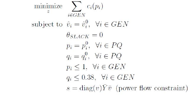
Note to expert: The optimization model above is for the problem and the data that follows is what will be required to evaluate the problem

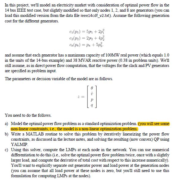
In this project, well model an electricity market with consideration of optimal power flow in the 14 bus IEEE test case, but slightly modified so that only nodes 1, 2, and 8 are generators (you can load this modified version from the data file ieee14cdf_v2.txt). Assume the following generation cost for the different generators. and assume that each generator has a maximum capacity of 100MW real power (which equals 1.0 in the units of the 14-bus example) and 38 MVAR reactive power (0.38 in problem units). We'll still assume, as in direct power flow computation, that the voltages for the slack and PV generators are specified as problem input The parameters or decision variable of the model are as follows. You need to do the follows. a) Model the optimal power flow problem as a standard optimization problem. (you will see some b) Write a MATLAB routine to solve this problem by iteratively linearizing the power flow non-linear constraints, i.e., the model is a non-linear optimization problem constraints, as discussed in the lecture notes, and solving the resulting (now convex) QP using YALMIP c) Using this solver, compute the LMPs at each node in the network. You can use numerical differentiation to do this (i.e., solve the optimal power flow problem twice, once with a slightly larger load, and compute the derivative of total cost with respect to this increase numerically. You'll want to explicitly separate out generator power and load power at the generation nodes (you can assume that all load power at these nodes is zero, but you'll still need to use this formulation for computing LMPs at the nodes). In this project, well model an electricity market with consideration of optimal power flow in the 14 bus IEEE test case, but slightly modified so that only nodes 1, 2, and 8 are generators (you can load this modified version from the data file ieee14cdf_v2.txt). Assume the following generation cost for the different generators. and assume that each generator has a maximum capacity of 100MW real power (which equals 1.0 in the units of the 14-bus example) and 38 MVAR reactive power (0.38 in problem units). We'll still assume, as in direct power flow computation, that the voltages for the slack and PV generators are specified as problem input The parameters or decision variable of the model are as follows. You need to do the follows. a) Model the optimal power flow problem as a standard optimization problem. (you will see some b) Write a MATLAB routine to solve this problem by iteratively linearizing the power flow non-linear constraints, i.e., the model is a non-linear optimization problem constraints, as discussed in the lecture notes, and solving the resulting (now convex) QP using YALMIP c) Using this solver, compute the LMPs at each node in the network. You can use numerical differentiation to do this (i.e., solve the optimal power flow problem twice, once with a slightly larger load, and compute the derivative of total cost with respect to this increase numerically. You'll want to explicitly separate out generator power and load power at the generation nodes (you can assume that all load power at these nodes is zero, but you'll still need to use this formulation for computing LMPs at the nodes)