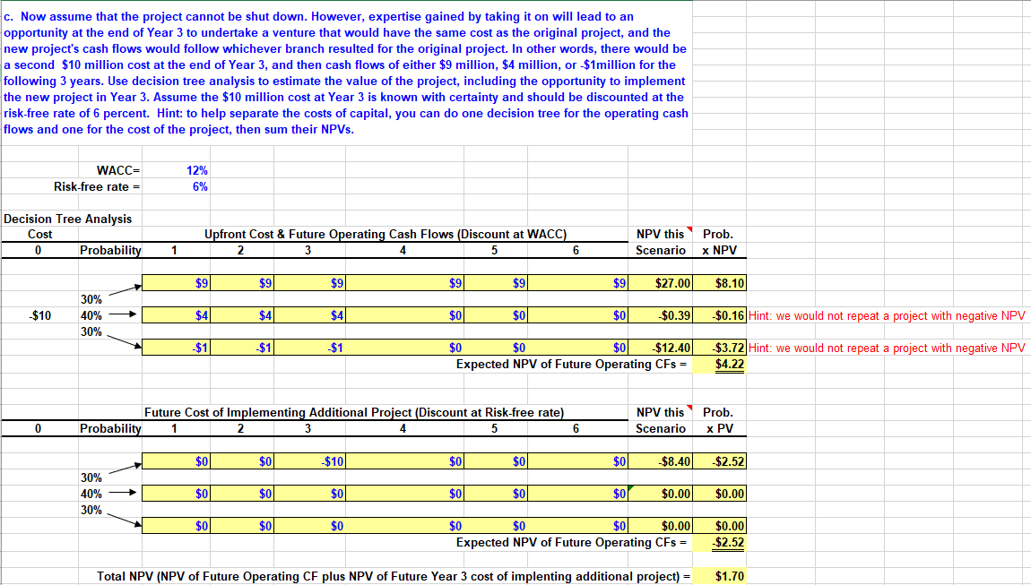
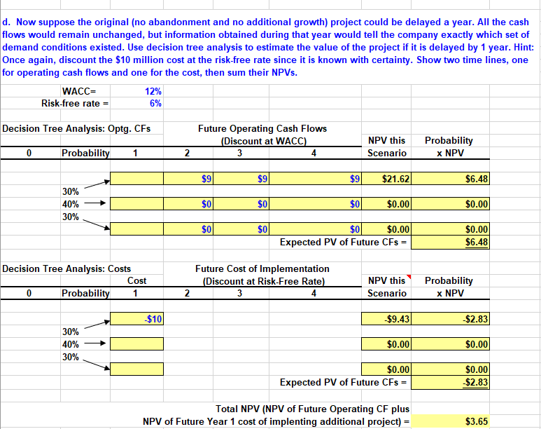
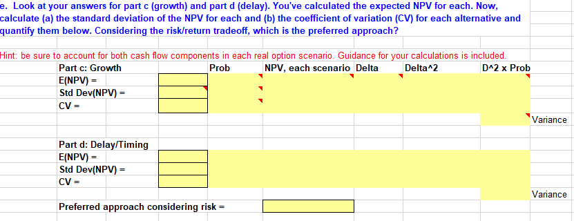
c. Now assume that the project cannot be shut down. However, expertise gained by taking it on will lead to an opportunity at the end of Year 3 to undertake a venture that would have the same cost as the original project, and the new project's cash flows would follow whichever branch resulted for the original project. In other words, there would be a second $10 million cost at the end of Year 3, and then cash flows of either $9 million, $4 million, or $1million for the following 3 years. Use decision tree analysis to estimate the value of the project, including the opportunity to implement the new project in Year 3. Assume the $10 million cost at Year 3 is known with certainty and should be discounted at the risk-free rate of 6 percent. Hint: to help separate the costs of capital, you can do one decision tree for the operating cash flows and one for the cost of the project, then sum their NPVs. WACC= Risk-free rate = 12% 6% Decision Tree Analysis Cost 0 Probability Upfront Cost & Future Operating Cash Flows (Discount at WACC) 2 3 4 5 6 NPV this Scenario Prob. x NPV 1 $9 $9| $91 $9 $90 $9 $27.00 $8.10) $10 30% 40% 30% $41 $4 $4 $0 $0 $0 $0.39 $0.16 Hint: we would not repeat a project with negative NPV $11 $1 $1 $0 $0 $0 $12.40 Expected NPV of Future Operating CFs = $3.72 Hint: we would not repeat a project with negative NPV $4.22 Future Cost of Implementing Additional Project (Discount at Risk-free rate) Probability 1 4 5 6 NPV this Scenario Prob. x PV 0 2 3 $0 $0 $100 $01 $0 $0 $8.40) $2.52 30% 40% 30% $0 $0 $0 $0 $0 $01 $0.00 $0.00 $0 $0 $0 $0 $0 $0 $0.00 Expected NPV of Future Operating CFs = $0.00 -$2.52 Total NPV (NPV of Future Operating CF plus NPV of Future Year 3 cost of implenting additional project) = $1.70 d. Now suppose the original (no abandonment and no additional growth) project could be delayed a year. All the cash flows would remain unchanged, but information obtained during that year would tell the company exactly which set of demand conditions existed. Use decision tree analysis to estimate the value of the project if it is delayed by 1 year. Hint: Once again, discount the $10 million cost at the risk-free rate since it is known with certainty. Show two time lines, one for operating cash flows and one for the cost, then sum their NPVs. WACC= 12% Risk-free rate = 6% Decision Tree Analysis: Optg. CFs Future Operating Cash Flows (Discount at WACC) 3 4 NPV this Scenario Probability 0 Probability 1 2 x NPV $90 $90 $9 $21.62 $6.48 30% 40% 30% $0 $0 $0 $0.00 $0.00 $0 $0 $0 $0.00 Expected PV of Future CFs = $0.00 $6.48 Decision Tree Analysis: Costs Cost 0 Probability 1 Future Cost of Implementation (Discount at Risk-Free Rate) 3 4 NPV this Scenario Probability x NPV 2 $100 $9.43 $2.83 30% 40% 30% $0.00 $0.00 $0.00 Expected PV of Future CFs = $0.00 $2.83 Total NPV (NPV of Future Operating CF plus NPV of Future Year 1 cost of implenting additional project) - $3.65 e. Look at your answers for part c (growth) and part d (delay). You've calculated the expected NPV for each. Now, calculate (a) the standard deviation of the NPV for each and (b) the coefficient of variation (CV) for each alternative and quantify them below. Considering the risk/return tradeoff, which is the preferred approach? Hint: be sure to account for both cash flow components in each real option scenario. Guidance for your calculations is included. Part c: Growth Prob NPV, each scenario Delta Delta2 D^2 x Prob E(NPV) = Std Dev(NPV) = CV- Variance Part d: Delay/Timing E(NPV) = Std Dev(NPV) = CV - Variance Preferred approach considering risk = c. Now assume that the project cannot be shut down. However, expertise gained by taking it on will lead to an opportunity at the end of Year 3 to undertake a venture that would have the same cost as the original project, and the new project's cash flows would follow whichever branch resulted for the original project. In other words, there would be a second $10 million cost at the end of Year 3, and then cash flows of either $9 million, $4 million, or $1million for the following 3 years. Use decision tree analysis to estimate the value of the project, including the opportunity to implement the new project in Year 3. Assume the $10 million cost at Year 3 is known with certainty and should be discounted at the risk-free rate of 6 percent. Hint: to help separate the costs of capital, you can do one decision tree for the operating cash flows and one for the cost of the project, then sum their NPVs. WACC= Risk-free rate = 12% 6% Decision Tree Analysis Cost 0 Probability Upfront Cost & Future Operating Cash Flows (Discount at WACC) 2 3 4 5 6 NPV this Scenario Prob. x NPV 1 $9 $9| $91 $9 $90 $9 $27.00 $8.10) $10 30% 40% 30% $41 $4 $4 $0 $0 $0 $0.39 $0.16 Hint: we would not repeat a project with negative NPV $11 $1 $1 $0 $0 $0 $12.40 Expected NPV of Future Operating CFs = $3.72 Hint: we would not repeat a project with negative NPV $4.22 Future Cost of Implementing Additional Project (Discount at Risk-free rate) Probability 1 4 5 6 NPV this Scenario Prob. x PV 0 2 3 $0 $0 $100 $01 $0 $0 $8.40) $2.52 30% 40% 30% $0 $0 $0 $0 $0 $01 $0.00 $0.00 $0 $0 $0 $0 $0 $0 $0.00 Expected NPV of Future Operating CFs = $0.00 -$2.52 Total NPV (NPV of Future Operating CF plus NPV of Future Year 3 cost of implenting additional project) = $1.70 d. Now suppose the original (no abandonment and no additional growth) project could be delayed a year. All the cash flows would remain unchanged, but information obtained during that year would tell the company exactly which set of demand conditions existed. Use decision tree analysis to estimate the value of the project if it is delayed by 1 year. Hint: Once again, discount the $10 million cost at the risk-free rate since it is known with certainty. Show two time lines, one for operating cash flows and one for the cost, then sum their NPVs. WACC= 12% Risk-free rate = 6% Decision Tree Analysis: Optg. CFs Future Operating Cash Flows (Discount at WACC) 3 4 NPV this Scenario Probability 0 Probability 1 2 x NPV $90 $90 $9 $21.62 $6.48 30% 40% 30% $0 $0 $0 $0.00 $0.00 $0 $0 $0 $0.00 Expected PV of Future CFs = $0.00 $6.48 Decision Tree Analysis: Costs Cost 0 Probability 1 Future Cost of Implementation (Discount at Risk-Free Rate) 3 4 NPV this Scenario Probability x NPV 2 $100 $9.43 $2.83 30% 40% 30% $0.00 $0.00 $0.00 Expected PV of Future CFs = $0.00 $2.83 Total NPV (NPV of Future Operating CF plus NPV of Future Year 1 cost of implenting additional project) - $3.65 e. Look at your answers for part c (growth) and part d (delay). You've calculated the expected NPV for each. Now, calculate (a) the standard deviation of the NPV for each and (b) the coefficient of variation (CV) for each alternative and quantify them below. Considering the risk/return tradeoff, which is the preferred approach? Hint: be sure to account for both cash flow components in each real option scenario. Guidance for your calculations is included. Part c: Growth Prob NPV, each scenario Delta Delta2 D^2 x Prob E(NPV) = Std Dev(NPV) = CV- Variance Part d: Delay/Timing E(NPV) = Std Dev(NPV) = CV - Variance Preferred approach considering risk =