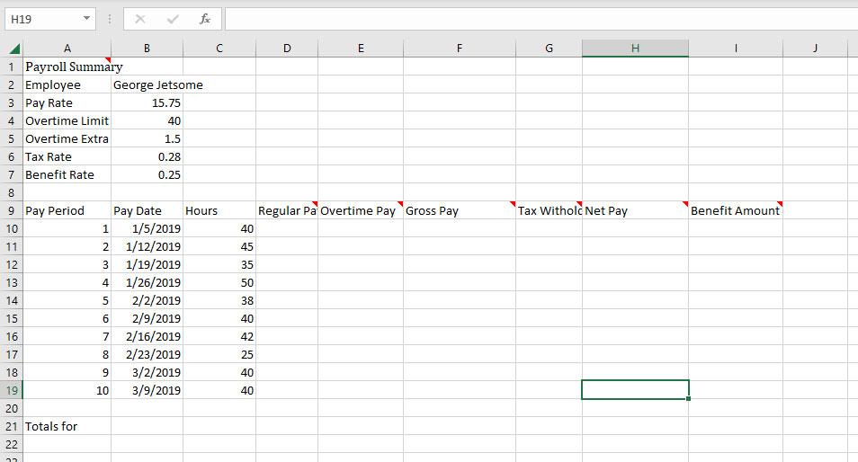
c. Provide formulas for regular pay (D10), overtime pay (E10), gross pay (F10), tax withholding (G10), net pay (H10), and benefit amount (I10) as indicated. In each formula, use an absolute reference for pay rate (B3), overtime limit (B4), overtime extra (B5), tax rate (B6), and benefit rate (B7) as needed. Compute regular pay (D10) as the minimum (MIN) of (hours (C10), overtime limit (B4)) times pay rate (B3). Use absolute references as indicated in (c). Compute overtime pay (E10) as the maximum (MAX) of (hours (C10) minus overtime limit (B4), 0) times pay rate (B3) times overtime extra (B5). Use absolute references as indicated in (c). Compute gross pay (F10) as regular pay (D10) plus overtime pay (E10). Compute tax withholding (G10) as gross pay (F10) times tax rate (B6). Use absolute references as indicated in (c). Compute net pay (H10) as gross pay (F10) minus tax withholding (G10). Compute benefit amount (I10) as gross pay (F10) times benefit rate (B7). Use absolute references as indicated in (c). d. Copy and paste D10:I10 to D11:I19. Before copying and pasting, make sure that you used absolute references when referencing cells B3:B7 in formulas in cells D10:I10. e. Make named ranges for hours (C10:C19), regular pay (D10:D19), overtime pay (E10:E19), gross pay (F10:F19), tax withholding (G10:G19), net pay (H10:H19), and benefit amount (I10:I19). Use the text in columns D9:I9 as names for each named range. For example, the name for C10:C19 will be Hours and D10:D19 will be Regular_Pay. Underscores should be used for spaces in names for ranges. You can create the named ranges quickly using Create from Selection in the Formulas menu. f. Modify cell A21 (Totals for ) with a formula using Totals for concatenated with employee name (B2). Use & for the concatenation operator. Use an absolute reference for employee name in the formula. Merge cell across cells A21:B21 and italicize the value in A21:B21. g. Enter a SUM function in cells C21:I21. Each function should use the named range for the cells in the same column of rows 10 to 19. For example, the formula in cell C21 should be =SUM(Hours). h. Format cells with dollar amounts (pay rate, regular pay, overtime pay, gross pay, net pay, benefit amount, and column totals) as Currency with two decimal places. Format sum of hours as a number without decimal digits. i. Apply cell styles as indicated in the following bullet points. Use cell style Heading 3 for cells A9:I9. Use cell style 20% Accent 1 for A2:A7. Use cell style Title for A1. Center and merge across cells A1:I1 j. Auto fit column width for any cells that do not fit into the default space except for the title centered in A1:I1. k. Format tax rate (B6) and benefit rate (B7) as percent with 2 decimal digits. l. Format summary totals (C21:I21) using the Output style.