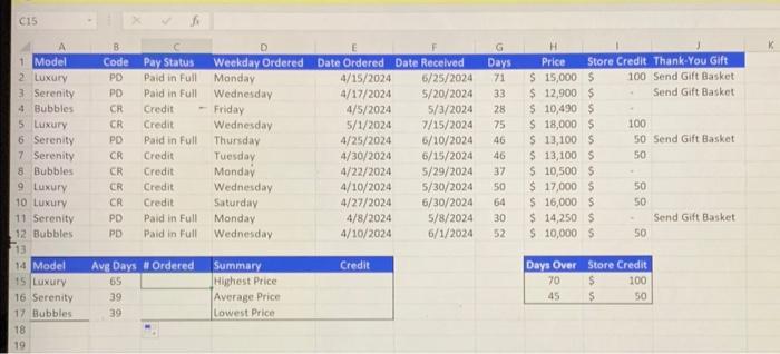
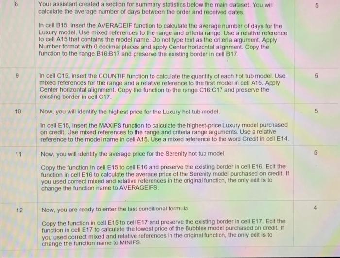
C15 8 Your assistant created a section for summary statistics below the main dataset. You will 5 calculate the average number of days between the order and received dates. In cell B15, insert the AVERAGEIF function to calculate the average number of days for the Luxury model. Use mixed references to the range and criteria range. Use a relative reference to cell A15 that contains the model name. Do not type text as the criteria argument. Apply Number format with 0 decimal places and apply Center horizontal alignment. Copy the function to the range B16:B17 and preserve the existing border in cell B17. In cell C15, insert the COUNTIF function to calculate the quantity of each hot tub model. Use 5 mixed references for the range and a relative reference to the first model in cell A15. Apply Center horizontal alignment. Copy the function to the range C16:C17 and preserve the existing border in cell C17. 10 Now, you will identify the highest price for the Luxury hot tub model. 5 In cell E15, insert the MAXIFS function to calculate the highest-price Luxury model purchased on credit. Use mixed references to the range and criteria range arguments. Use a relative reference to the model name in cell A15. Use a mixed reference to the word Credit in cell E14. 11 Now, you will identify the average price for the Serenity hot tub model. 5 Copy the function in cell E15 to cell E16 and preserve the existing border in cell E16. Edit the function in cell E16 to calculate the average price of the Serenity model purchased on credit. If you used correct mixed and relative references in the original function, the only edit is to change the function name to AVERAGEIFS. 12 Now, you are ready to enter the last conditional formula. 4 Copy the function in cell E15 to cell E17 and preserve the existing border in cell E17. Edit the function in cell E17 to calculate the lowest price of the Bubbles model purchased on credit. If you used correct mixed and relative references in the original function, the only edit is to change the function name to MINIFS