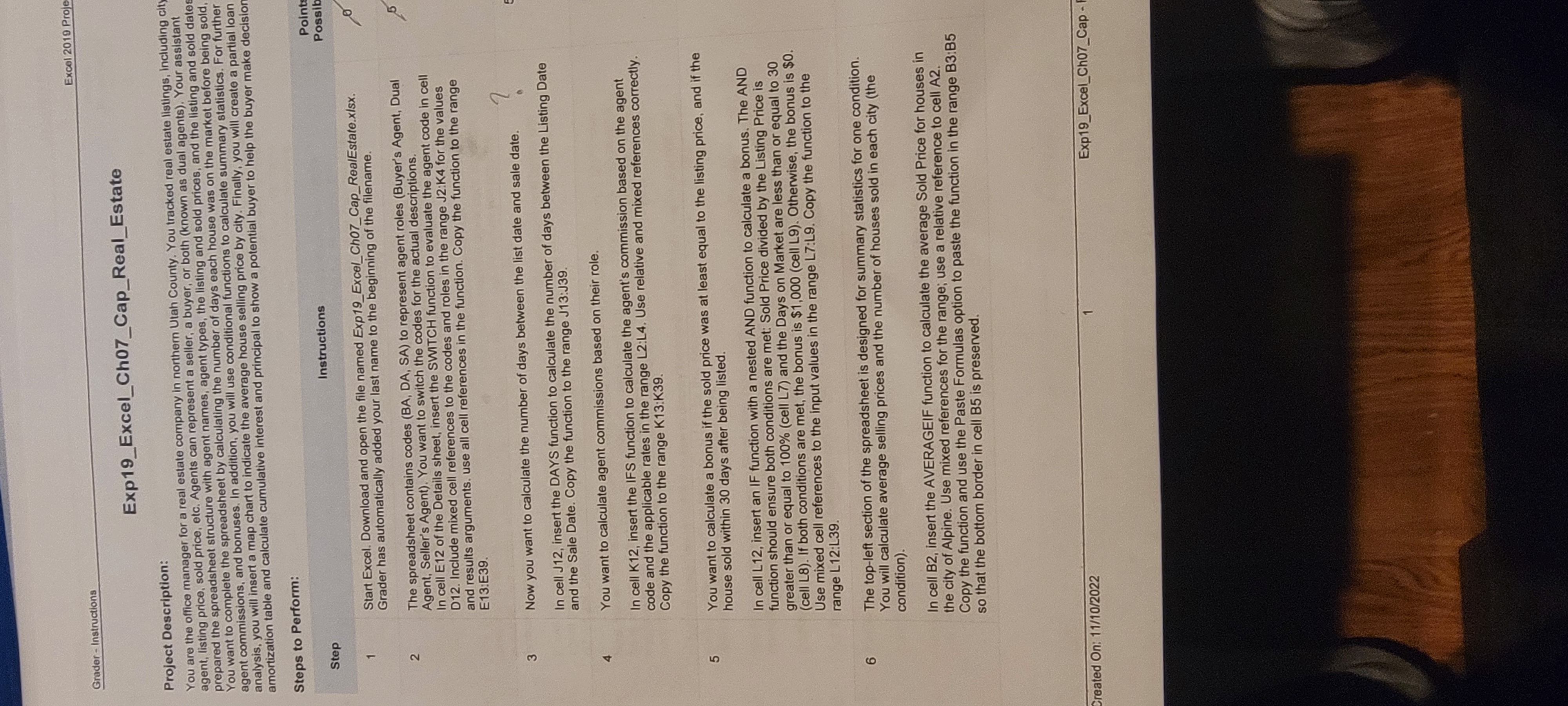
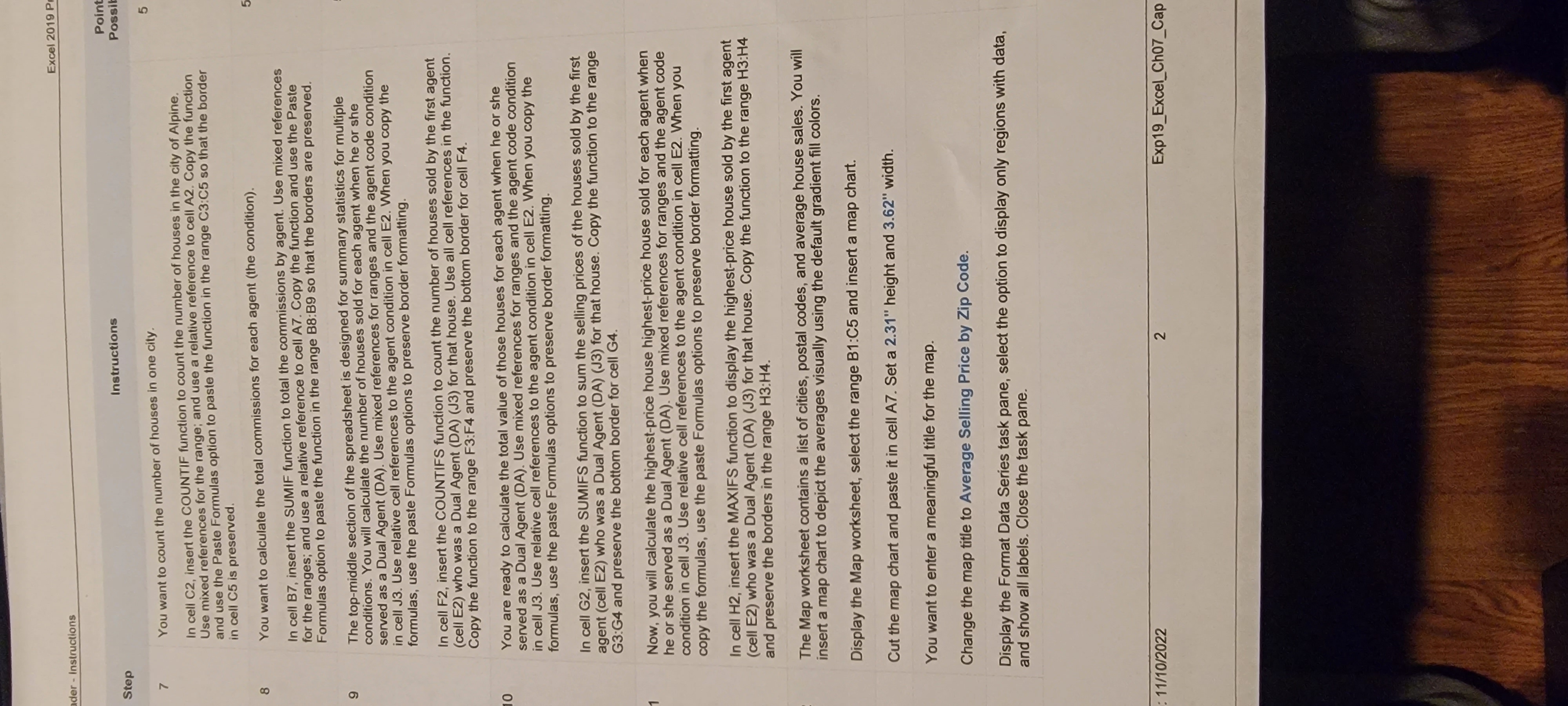
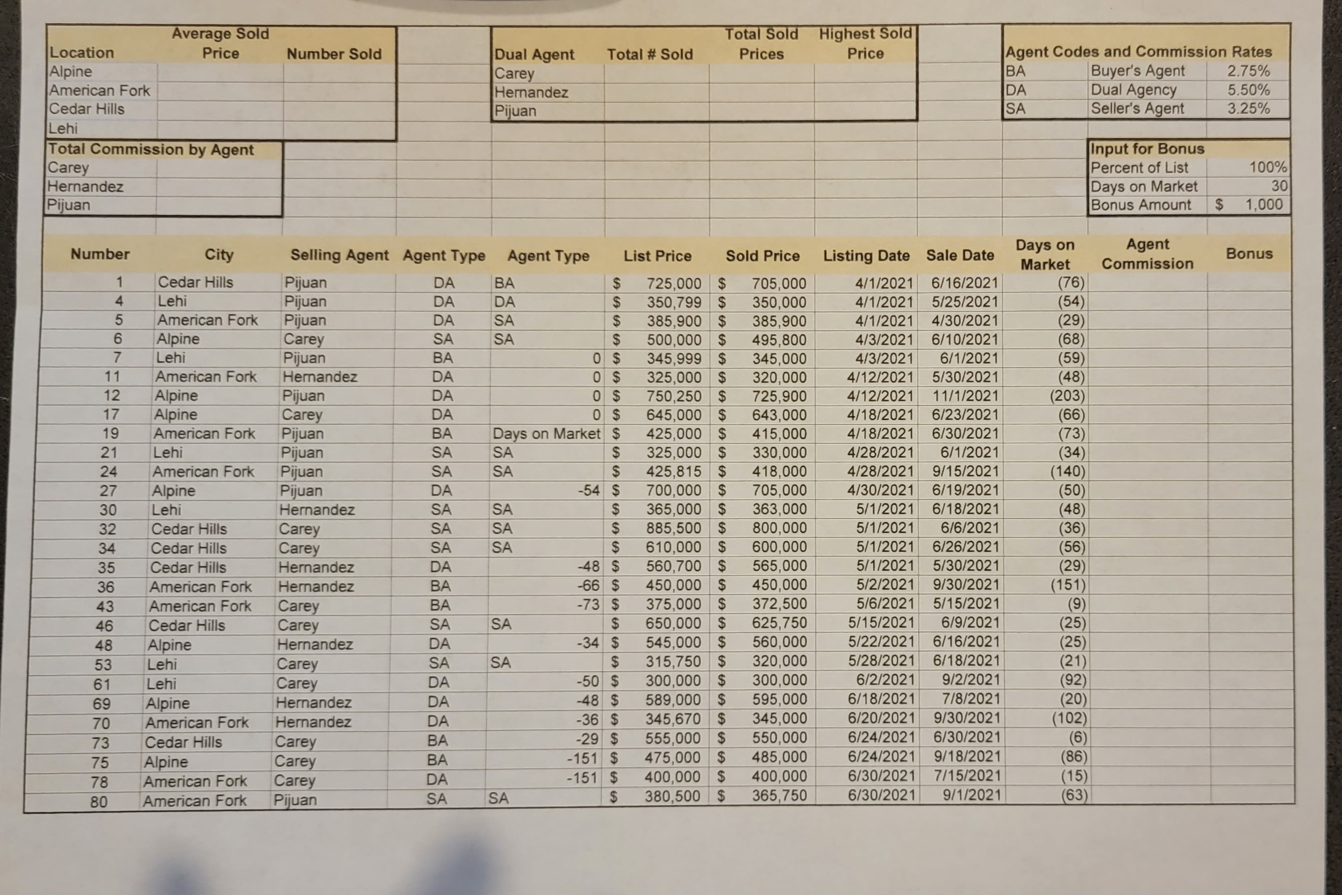
Excel 2019 Proje der - Instructions Points Step Instructions Possible 16 You are ready to start completing the loan amortization table. 5 Display the Loan worksheet. In cell B8, type a reference formula to cell B1. The balance before the first payment is identical to the loan amount. Do not type the value; use the cell reference instead. In cell B9, subtract the principal from the beginning balance on the previous row. Copy the formula to the range B10:B19. 17 Now, you will calculate the interest for the first payment. 5 In cell C8, calculate the interest for the first payment using the IPMT function. Copy the function to the range C9:C19. 18 Next, you will calculate the principal paid. 5 In cell D8, calculate the principal paid for the first payment using the PPMT function. Copy the function to the range D9:D19. Rows 21-23 contain a summary section for cumulative totals after the first year. In cell B22, insert the CUMIPMT function that calculates the cumulative interest after the first year. Use references to cells A8 and A19 for the period arguments. The next summary statistic will calculate the principal paid after the first year. In cell B23, insert the CUMPRINC function that calculates the cumulative principal paid after the first year. Use references to cells A8 and A19 for the period arguments. Rows 25-28 contain a section for what-if analysis. In cell B27, use the RATE financial function to calculate the periodic rate using $1,400 as the monthly payment (cell B26), the NPER, and loan amount in the original input section. In cell B28, calculate the APR by multiplying the monthly rate (cell B27) by 12. Create a footer on all three worksheets with your name on the left side, the sheet name code in the center, and the file name code on the right side of each worksheet. Save and close Exp19_Excel_Ch07_Cap_RealEstate.xIsx. Exit Excel. Submit the file as directed. Total Points 1/10/2022 3 Exp19_Excel_Ch07_CapGrader - Instructions Excel 2019 Proj Exp19_Excel_Ch07_Cap_Real_Estate Project Description: You are the office manager for a real estate company in northern Utah County. You tracked real estate listings, including cit agent, listing price, sold price, etc. Agents can represent a seller, a buyer, or both (known as dual agents). Your assistant prepared the spreadsheet structure with agent names, agent types, the listing and sold prices, and the listing and sold dates You want to complete the spreadsheet by calculating the number of days each house was on the market before being sold agent commissions, and bonuses. In addition, you will use conditional functions to calculate summary statistics. For further analysis, you will insert a map chart to indicate the average house selling price by city. Finally, you will create a partial loan amortization table and calculate cumulative interest and principal to show a potential buyer to help the buyer make decision Steps to Perform: Point Step Instructions Possib Start Excel. Download and open the file named Exp19_Excel_Ch07_Cap_RealEstate.xisx. Grader has automatically added your last name to the beginning of the filename. 2 The spreadsheet contains codes (BA, DA, SA) to represent agent roles (Buyer's Agent, Dual Agent, Seller's Agent). You want to switch the codes for the actual descriptions. In cell E12 of the Details sheet, insert the SWITCH function to evaluate the agent code in cell D12. Include mixed cell references to the codes and roles in the range J2:K4 for the values and results arguments. use all cell references in the function. Copy the function to the range E13:E39. 3 Now you want to calculate the number of days between the list date and sale date. In cell J12, insert the DAYS function to calculate the number of days between the Listing Date and the Sale Date. Copy the function to the range J13:J39. You want to calculate agent commissions based on their role. In cell K12, insert the IFS function to calculate the agent's commission based on the agent code and the applicable rates in the range L2:L4. Use relative and mixed references correctly. Copy the function to the range K13:K39. 5 You want to calculate a bonus if the sold price was at least equal to the listing price, and if the house sold within 30 days after being listed. In cell L12, insert an IF function with a nested AND function to calculate a bonus. The AND function should ensure both conditions are met: Sold Price divided by the Listing Price is greater than or equal to 100% (cell L7) and the Days on Market are less than or equal to 30 (cell L8). If both conditions are met, the bonus is $1,000 (cell L9). Otherwise, the bonus is $0. Use mixed cell references to the input values in the range L7:L9. Copy the function to the range L12:L39. 6 The top-left section of the spreadsheet is designed for summary statistics for one condition. You will calculate average selling prices and the number of houses sold in each city (the condition). In cell B2, insert the AVERAGEIF function to calculate the average Sold Price for houses in the city of Alpine. Use mixed references for the range; use a relative reference to cell A2. Copy the function and use the Paste Formulas option to paste the function in the range B3:B5 so that the bottom border in cell B5 is preserved. Created On: 11/10/2022 Exp19_Excel_Ch07_CapExcel 2019 der - Instructions Instructions Point Step Possil 7 You want to count the number of houses in one city. 5 In cell C2, insert the COUNTIF function to count the number of houses in the city of Alpine. Use mixed references for the range; and use a relative reference to cell A2. Copy the function and use the Paste Formulas option to paste the function in the range C3:C5 so that the border in cell C5 is preserved. 8 You want to calculate the total commissions for each agent (the condition). In cell B7, insert the SUMIF function to total the commissions by agent. Use mixed references for the ranges; and use a relative reference to cell A7. Copy the function and use the Paste Formulas option to paste the function in the range B8:B9 so that the borders are preserved. The top-middle section of the spreadsheet is designed for summary statistics for multiple conditions. You will calculate the number of houses sold for each agent when he or she served as a Dual Agent (DA). Use mixed references for ranges and the agent code condition in cell J3. Use relative cell references to the agent condition in cell E2. When you copy the formulas, use the paste Formulas options to preserve border formatting. In cell F2, insert the COUNTIFS function to count the number of houses sold by the first agent (cell E2) who was a Dual Agent (DA) (J3) for that house. Use all cell references in the function. Copy the function to the range F3:F4 and preserve the bottom border for cell F4. 10 You are ready to calculate the total value of those houses for each agent when he or she served as a Dual Agent (DA). Use mixed references for ranges and the agent code condition in cell J3. Use relative cell references to the agent condition in cell E2. When you copy the formulas, use the paste Formulas options to preserve border formatting. In cell G2, insert the SUMIFS function to sum the selling prices of the houses sold by the first agent (cell E2) who was a Dual Agent (DA) (J3) for that house. Copy the function to the range G3:G4 and preserve the bottom border for cell G4. Now, you will calculate the highest-price house highest-price house sold for each agent when he or she served as a Dual Agent (DA). Use mixed references for ranges and the agent code condition in cell J3. Use relative cell references to the agent condition in cell E2. When you copy the formulas, use the paste Formulas options to preserve border formatting. In cell H2, insert the MAXIFS function to display the highest-price house sold by the first agent (cell E2) who was a Dual Agent (DA) (J3) for that house. Copy the function to the range H3:H4 and preserve the borders in the range H3:H4. The Map worksheet contains a list of cities, postal codes, and average house sales. You will insert a map chart to depict the averages visually using the default gradient fill colors. Display the Map worksheet, select the range B1:C5 and insert a map chart. Cut the map chart and paste it in cell A7. Set a 2.31" height and 3.62" width. You want to enter a meaningful title for the map. Change the map title to Average Selling Price by Zip Code. Display the Format Data Series task pane, select the option to display only regions with data, and show all labels. Close the task pane. 11/10/2022 2 Exp19_Excel_Ch07_CapAverage Sold Total Sold Highest Sold Location Price Number Sold Dual Agent Total # Sold Prices Price Agent Codes and Commission Rates Alpine Carey BA Buyer's Agent 2.75% American Fork Hernandez DA Dual Agency 5.50% Cedar Hills Pijuan SA Seller's Agent 3.25% Lehi Total Commission by Agent Input for Bonus Carey Percent of List 100% Hernandez Days on Market 30 Pijuan Bonus Amount $ 1,000 Sold Price Listing Date Sale Date Days on Agent Number City Selling Agent Agent Type Agent Type List Price Bonus Market Commission Cedar Hills Pijuan DA BA $ 725,000 $ 705,000 4/1/2021 6/16/2021 (76) Lehi Pijuan DA DA 350,799 $ 350,000 4/1/2021 5/25/2021 (54) American Fork Pijuan DA SA 385,900 $ 385,900 4/1/2021 4/30/2021 (29) Alpine Carey SA SA $ 500,000 495,800 4/3/2021 6/10/2021 (68) 7 Lehi Pijuan BA OS 345,999 345,000 4/3/2021 6/1/2021 (59) 11 American Fork Hernandez DA 325,000 $ 320,000 4/12/2021 5/30/2021 (48) 12 Alpine Pijuan DA O $ 750,250 $ 725,900 4/12/2021 11/1/2021 203 17 Alpine Carey DA O $ 645,000 $ 643,000 4/18/2021 6/23/2021 66) 19 American Fork Pijuan BA Days on Market $ 425,000 $ 415,000 4/18/2021 6/30/2021 (73) 21 Lehi Pijuan SA SA 325,000 $ 330,000 4/28/2021 6/1/2021 (34) 24 American Fork Pijuan SA SA 425, 815 $ 418,000 4/28/2021 9/15/2021 (140) 27 Alpine Pijuan DA 54 $ 700,000 705,000 4/30/2021 6/19/2021 (50) 30 Lehi Hernandez SA SA 365,000 363,000 5/1/2021 6/18/2021 (48) 32 Cedar Hills Carey SA SA 885,500 800,000 5/1/2021 6/6/2021 (36) 34 Cedar Hills Carey SA SA 610,000 600,000 5/1/2021 6/26/2021 56) 35 Cedar Hills Hernandez DA -48 $ 560,700 565,000 5/1/2021 5/30/2021 (29) 36 American Fork Hernandez BA -66 $ 450,000 450,000 5/2/2021 9/30/2021 (151) 43 American Fork Carey BA -73 $ 375,000 372,500 5/6/2021 5/15/2021 (9) 46 Cedar Hills Carey SA SA $ 650,000 625,750 5/15/2021 6/9/2021 25) 48 Alpine Hernandez DA 34 $ 545,000 $ 560,000 5/22/2021 6/16/2021 (25) 53 Lehi Carey SA SA $ 315,750 $ 320,000 5/28/2021 6/18/2021 (21) 61 Lehi Carey DA 50 $ 300,000 300,000 6/2/2021 9/2/2021 (92) 69 Alpine Hernandez DA -48 $ 589,000 595,000 6/18/2021 7/8/2021 (20) 70 American Fork Hernandez DA 36 $ 345,670 345,000 6/20/2021 9/30/2021 (102 73 Cedar Hills Carey BA -29 $ 555,000 550,000 6/24/2021 6/30/2021 (6) 75 Alpine Carey BA -151 $ 475,000 $ 485,000 6/24/2021 9/18/2021 (86) 78 American Fork Carey DA -151 $ 400,000 $ 400,000 6/30/2021 7/15/2021 (15) 80 American Fork Pijuan SA SA $ 380,500 $ 365,750 6/30/2021 9/1/2021 (63)