Can I get help with this, I also need the formulas for the work sheet.

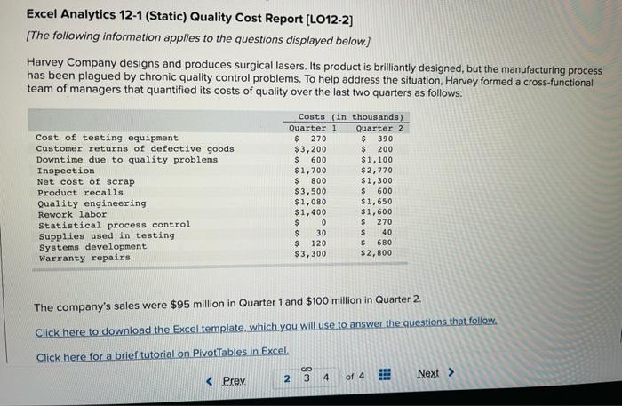
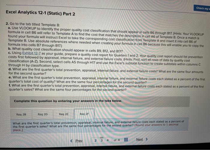
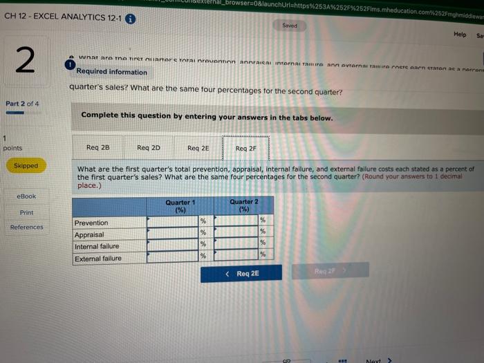
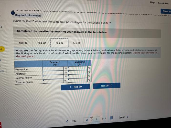
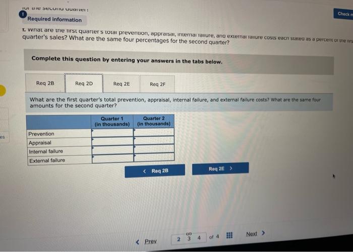
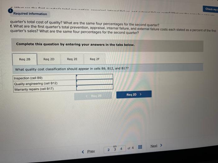
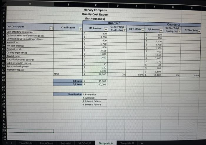
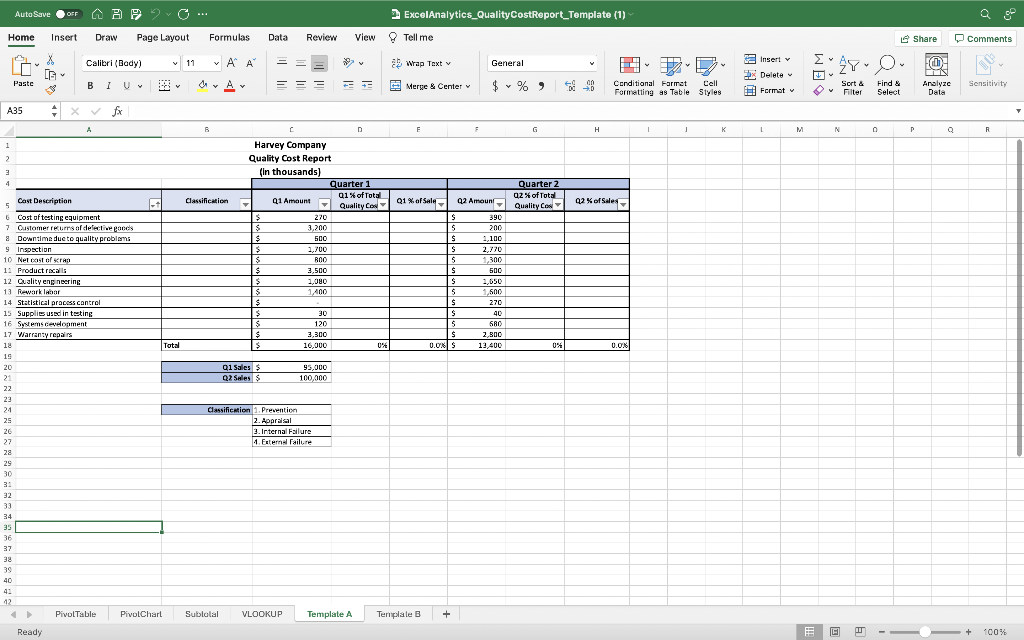
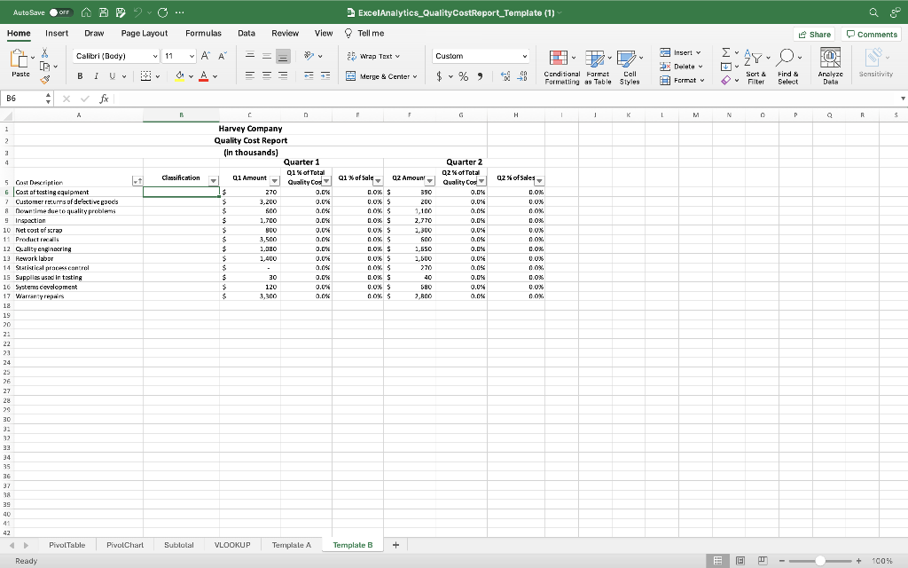
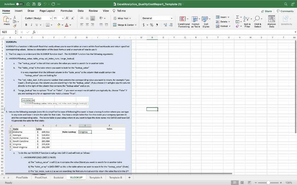
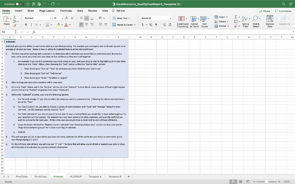
AutoSave IF A ExcelAnalytics_QualityCostReport_Template (1) View Tell me Home Insert Draw Page Layout Formulas Data Review Share Comments Calibri (Bady) Insert v 11 A u a Wrap Text v General ' 480 Fech [G Delete Paste BIU A VA = = - - Merge & Center $ % Conditional Format Cell Formatting as Table Styles Sort & Filter Format w Find & Select Analyze Dala Sensitivity A35 fx B D F G H 1 1 1 M N P Q R 1 2 3 4. 01% of Total 21%of Sale Quarter 2 02% of Total Cast Description Classification Q1 % Q2 Amor Quality Con Amount 92% of Sales Harvey Company Quality Cost Report (in thousands) Quarter 1 41 Amount Quality Cox $ 270 $ 3,200 $ 500 $ 1,700 $ 800 $ 3,500 $ 1,080 $ 1,400 $ $ 30 $ 120 $ 3,300 $ 16,000 074 $ S $ $ 5 $ $ 5 $ $ 5 $ 0.OS 390 200 1,100 2,770 1,300 500 1,650 1,500 270 an 40 580 2.800 13,400 Total 0.0 6 Cost of testing equipment 7 Customer resursafdeliwood's 3 Downtime due to quality problems 9 Inspection 10 Nel cast of cran 11 Product recalls 12 Quality engineering 13 Rewarkleber 14 Statistical process control 15 Supplies used in testing int 16 Systems cevelopment 17 Warranty repairs 18 19 20 21 22 23 24 25 26 27 28 29 30 3: 32 33 34 Q1 Sales $ Q2 Sales 95,000 100,000 Classification 1. Prevention 2. Appraisal 2.Internal Failure 1. External Failure 36 37 39 40 12 Pivo Table PivolChart Sublolal VLDDRUP Template A Template + Ready C - + 100% AutoSave IF A Home Insert Draw Page Layout Formulas Data Review Share 0 Comments ExcelAnalytics_QualityCostReport_Template (1) View Tell me ah Wrap Text v Custom - - Merge & Center v Conditional Farret Cell Formatting as Table Styles Calibri (Bady) v 11 ~ Al A , X [G Fah Insert v Delete Format 2Y-. AY Paste B 1 VA = = Sort & Filter Find & Select Analyze Data Sensitivity B6 A xv fx T A B D E F G H 1 1 1 M N 0 P Q R s 1 2 3 4 Classification Q1 Amount - Quality Con 6 Harvey Company Quality Cost Report (In thousands) Quarter 1 Q1% of Total 01 $ 270 0.0% $ 3,200 0.0% $ 500 0.0% $ 1.700 0.0% $ 900 0.0% $ S 3,500 0.0% $ 1.380 0.0% % $ 1,400 0.0 $ 0.0% $ 30 0.0% $ 120 0.0% $ 3,300 0.0% 91% of Sale 02 Amount 00 $ 390 0.0% 5 200 0.09. S 1,100 0.0% $ $ 2,770 0.06 $ 1,300 0.0% 5 500 0.0% $ $ 1.550 0.06 $ 1,600 0.0.6 270 0.0% $ $ 40 0.06 $ 640 0.0%. $ 2,000 Quarter 2 02% of Total Quality Cos 0.0% 0.0% 0.0% 0.0% % 0.0 0.0% 0.0% 0.0 0.0% 0.0% % 0.0 0.0% 02% of Sales 0.0% 0.0% 0.0% . 0.0% 0.0.6 0.0% 0.0% 0.0% 0.0%. 0.08 VOX 0.0%. 5 Cast Description E Cost of testing equipment 7 Customer resurrs of delective goods newntimeluet quality problems 9 Inspection 10 Net cost of scrap 11 Products 12 Quality engineering 13 Rework labor 14 Statistical process control 15 Supplies used in testing 16 Systems cevelopment 17 Warranty repairs 18 19 20 2: 22 23 24 25 26 27 28 20 30 3 32 33 34 35 36 37 38 39 40 41 42 Pivo Table PivolChart Sublolal VLDDRUP Template Template B + Ready 100% AutoSave OFF A Home Insert Draw Page Layout Formulas Share 0 Comments ExcelAnalytics_QualityCostReport_Template (1) Data Review View Tell me ab Wrap Textv General = = - $ % Merge & Center 90 Cell Conditional Format Formatting as Table Styles Calibri (Bady) v 11 ~ A , 1 X [G Insert v Delete Format AY Fah @ Paste B 1 A Sort & O Filter Find & Select Analyze Data Sensitivity N23 N M N P Q R s s T T U V w X Z AA 2 h. c A D E G H 1 K 1 VLOOKUPs 2 3 VLOOKUP is a function in Micrasoft Excel that easily alloras yau to search tables ar sheets within Excel workeaks and return specified 4 Corresponding values. Below is a description of the Excel formua and an example of how to use it: 5 1. The first step is to understand the VLOOKUP furction itself. The VLOOKUP Funktion has the following arguments: 2. =VLOOKUPlookup_value, table_array, col_index_rum, (range_laskual 8 The "ookup_value is the cell that contains the value you want to search for in another table 9 The table_array" is the table where you want to look for the lookup_value" 10 11 It is very important that the leftmost column in the table_array is the column that would contain the 12 lookup_value you se look relor 13 14 C. The "col_index_num, is the column number that contains the corresponding value you want to return, for example if you input 1. It wil gve you the calumn you are searching in for the "lookup_value", if you choose 2 I will give you the column 15 directly to the right of the column that contains the 'lockup value and so on. 16 17 4. rere_lookup has to options "True" ar "False". If you want an exact march which you typically lo, cheese "False ir 18 you are looking only tor an approximate match.choose "truc". 19 20 -L00K LIP || 21 VLOOKUP lookup value, table array, colinde numrage lookup 22 23 24. 3. Tesco the following seample note this is smalled for ease of following you want to have a lookup Nunction where you can type 25 in any state and have itrenurn the sales for that state. You have a simple table that is the states your company operates in 26 and the corresponding sales. The belon table as your setup where in you want to type the state name into Cell E2 and have Cell 27 F2 generate the sales for that state: 28 A B D F 29 1 1 State Sales 30 2 Alabama $ 169,511 State Lookup Virginia 3 Georgia $ 128,652 32 4 North Carolina $ 244,164 33 5 South Carolina $ 283,094 34 6 Virginia $ 205,626 35 7 West Virginia $ 196,359 36 37 To do this pur VLOOKUP function is will go into Cell F2 and will look as follows: 38 1. -VLOOKUPE2,$A$1$B$7,2,FALSE) 39 40 al The Hookup_value" s cell 2 as it contains the value Statel you want to search for in anuther table 41 The table_array($A$1:$A$7 as this the table where we want to search for the 'lookup_value" (State) 42 43 c) The colindex_num is 2 as we are scarching the first column but want to turn the value found in the ra [ 4 Pivot Table PivolChart Sublolal VLOOKUP Template Template B + Ready w 100% Share 0 Comments , Insert v Delete Format AY Fah Sort & O Filter Find & Select Analyze Data Sensitivity P U V w X Z AA 1 4 6 ? AutoSave IF AAP ExcelAnalytics_QualityCostReport_Template (1) Home Insert Draw Page Layout Formulas Data Review View Tell me X Symbol v 12 v AP AM 92 ab Wrap Textv General [G Paste B 1 U - A - - Merge & Center $ % 90 Conditional Format Cell Formatting as Table Styles A1 x A C D F G H 1 K N N Q R s S Subtotals: 2 Subtotals give you the ability to summarize data ay a specified grouping. For example you could get a sum of all sales by year ar an 3 average of all sales by state. Below is how to utilize the Subtotal feature within Microsoft Excel 5 1 . The first step when working with subtotals is to determine which attribute you would like to summarize your data tyle yes, state, store, etc) then sort your data on that attribute so they are isted together . For cample if you want to summarize your data based on year, sort your data by year by highlighting all of your data, a clicking on the Data ribbon, then chocoing the "Sort" button within the sort & Filter" section 9 10 1. Then choose to "Sort Year" for whatever you have titled the year columnas 11 2. Then choos ng to sort on "Cell Values 12 13 3. Then choose to "Order Smallest ta largest 14 2 2. After sorting your data click anywhere within your data 15 10 3. Gota the Data ribbon and in the "Ciline section click the "Subtotal" button INote: some versions of Excel right require 17 you to click on the Outline dropdown Then select "Subtotal") 12 4. within the "Subtotal wdow, you have the following options: 19 20 For "Ateach change in you should select the value you want a summarize by. Following the above example here it would be "Year 2 22 b. b. For "Use function you are able to choose a variety of summarization with "Sum" and "Pwerage" being the mos. 23 corrmon. For this example, set this input to Sum 24 c. For "Add subtotal to you should check the bar nest to any numerical fields you would like to hawe added together for 25 your specific summary group. For example you may have columns for sales, expenses, and quantity sold that you 26 want to summarize for each year. If this is the case you would show a check next to each of those attributes. 27 28 Leave the boxes checked for "Replace current subtatals and "Summary below data and do not deck the box for 20 *Page break between grous for a dean rearing of subtatals 30 Click OK 31 32 5. 5. This will now give you an output where you have summary subtotal for all the attributes you chose se summarize the 33 specified grouping (i.e.year) 34 G. On the left hanc side of Excel you will now see and buttons that will allow you to shrink or expand your cata to show 35 all of the data with subtotals or just the subtotals themselves 36 32 38 35 40 d. 42 43 24 PivolTable PivolChart Sublolal VLCDKUP Templale A Templates + Ready Cu + 100% Excel Analytics 12-1 (Static) Quality Cost Report [LO12-2) [The following information applies to the questions displayed below) Harvey Company designs and produces surgical lasers. Its product is brilliantly designed, but the manufacturing process has been plagued by chronic quality control problems. To help address the situation, Harvey formed a cross-functional team of managers that quantified its costs of quality over the last two quarters as follows: Cost of testing equipment Customer returns of defective goods Downtime due to quality problems Inspection Net cost of scrap Product recalls Quality engineering Rework labor Statistical process control Supplies used in testing Systems development Warranty repairs Costs (in thousands) Quarter 1 Quarter 2 $ 270 $ 390 $3,200 $ 200 $ 600 $1,100 $1,700 $2,770 $ 800 $1,300 $3,500 $ 600 $1,080 $1,650 $1,400 $1,600 $ 0 $ 270 $ 30 $ 40 $ 120 $ 680 $3,300 $2,800 The company's sales were $95 million in Quarter 1 and $100 million in Quarter 2. Click here to download the Excel template, which you will use to answer the questions that follow. Click here for a brief tutorial on Pivot Tables in Excel 2 3 4 Check my Excel Analytics 12-1 (Static) Part 2 2. Go to the tab titled Template B: a. Use VLOOKUP to identify the proper quality cost classification that should appear in cells B6 through B17. (Hints: Your VLOOKUP formula in cell B6 will refer to Template A to find the cost that matches the description in cell A6 of Template B. Once a match is found your formula will instruct Excel to take the corresponding cost classification from Template A and Insert it into cell B6 of Template B. Use absolute references where needed when creating your formula in cell B6 because this will enable you to copy the formula into cells B7 through B17.) b. What quality cost classification should appear in cells B9, B12, and B17? c. Using Exhibit 12-7 as your guide, prepare a quality cost report for Quarters 1 and 2. Your quality cost report should list prevention costs first followed by appraisal, internal failure, and external fallure costs. (Hints: First, sort all rows of data by quality cost classification (A-2). Second, select cells A5 through H17 and use the Excel's subtotal function to create subtotals within columns through H by classification type. d. What are the first quarter's total prevention, appraisal, internal failure, and external failure costs? What are the same four amounts for the second quarter? e. What are the first quarter's total prevention, appraisal, internal failure, and external failure costs each stated as a percent of the first quarter's total cost of quality? What are the same four percentages for the second quarter? f. What are the first quarter's total prevention, appraisal, internal failure, and external failure costs each stated as a percent of the first quarter's sales? What are the same four percentages for the second quarter? Complete this question by entering your answers in the tabs below. Reg 28 Reg 2D Req 2E Req 2F What are the first quarter's total prevention, appraisal, internal failure, and external failure costs each stated as a percent of the first quarter's sales? What are the same four percentages for the second quarter? (Round your answers to 1 decimal place.) browser=0&launchUriahttps%253A252F%252Fims.mheducation.com%252Fmghmiddlewar CH 12 - EXCEL ANALYTICS 12-16 Served Help Sa 2 What are no tirer innere TATAI nrovannen an internal annararname rere an earn a norra Required information quarter's sales? What are the same four percentages for the second quarter? Part 2 of 4 Complete this question by entering your answers in the tabs below. 1 points Reg 28 Reg 2D Reg 2E Reg 2F Skipped What are the first quarter's total prevention, appraisal, internal failure, and external failure costs each stated as a percent of the first quarter's sales? What are the same four percentages for the second quarter? (Round your answers to 1 decimal place.) eBook Quarter 2 Print % References Prevention Appraisal Internal failure External failure Quarter 1 (%) % % % % % % % % Next > sm 2 N 3 4 of 4 ! Next > 3 4 of 4 !!! Next > Son 2. 3 4 of 4 ! Check my Excel Analytics 12-1 (Static) Part 2 2. Go to the tab titled Template B: a. Use VLOOKUP to identify the proper quality cost classification that should appear in cells B6 through B17. (Hints: Your VLOOKUP formula in cell B6 will refer to Template A to find the cost that matches the description in cell A6 of Template B. Once a match is found your formula will instruct Excel to take the corresponding cost classification from Template A and Insert it into cell B6 of Template B. Use absolute references where needed when creating your formula in cell B6 because this will enable you to copy the formula into cells B7 through B17.) b. What quality cost classification should appear in cells B9, B12, and B17? c. Using Exhibit 12-7 as your guide, prepare a quality cost report for Quarters 1 and 2. Your quality cost report should list prevention costs first followed by appraisal, internal failure, and external fallure costs. (Hints: First, sort all rows of data by quality cost classification (A-2). Second, select cells A5 through H17 and use the Excel's subtotal function to create subtotals within columns through H by classification type. d. What are the first quarter's total prevention, appraisal, internal failure, and external failure costs? What are the same four amounts for the second quarter? e. What are the first quarter's total prevention, appraisal, internal failure, and external failure costs each stated as a percent of the first quarter's total cost of quality? What are the same four percentages for the second quarter? f. What are the first quarter's total prevention, appraisal, internal failure, and external failure costs each stated as a percent of the first quarter's sales? What are the same four percentages for the second quarter? Complete this question by entering your answers in the tabs below. Reg 28 Reg 2D Req 2E Req 2F What are the first quarter's total prevention, appraisal, internal failure, and external failure costs each stated as a percent of the first quarter's sales? What are the same four percentages for the second quarter? (Round your answers to 1 decimal place.) browser=0&launchUriahttps%253A252F%252Fims.mheducation.com%252Fmghmiddlewar CH 12 - EXCEL ANALYTICS 12-16 Served Help Sa 2 What are no tirer innere TATAI nrovannen an internal annararname rere an earn a norra Required information quarter's sales? What are the same four percentages for the second quarter? Part 2 of 4 Complete this question by entering your answers in the tabs below. 1 points Reg 28 Reg 2D Reg 2E Reg 2F Skipped What are the first quarter's total prevention, appraisal, internal failure, and external failure costs each stated as a percent of the first quarter's sales? What are the same four percentages for the second quarter? (Round your answers to 1 decimal place.) eBook Quarter 2 Print % References Prevention Appraisal Internal failure External failure Quarter 1 (%) % % % % % % % % Next > sm 2 N 3 4 of 4 ! Next > 3 4 of 4 !!! Next > Son 2. 3 4 of 4 !