

Question: Can I have the code to input these values and plot it like the graph below but on mathematica with error bars and a legend
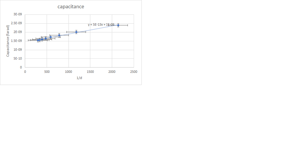
Can I have the code to input these values and plot it like the graph below but on mathematica with error bars and a legend and x and y titles?? 1/d (x axis) capacitance(y axis)
2139.037433 2.4E-09 1176.470588 2.01E-09 784.3137255 1.82E-09 588.2352941 1.72E-09 470.5882353 1.64E-09 392.1568627 1.6E-09 336.1344538 1.56E-09 294.1176471 1.54E-09
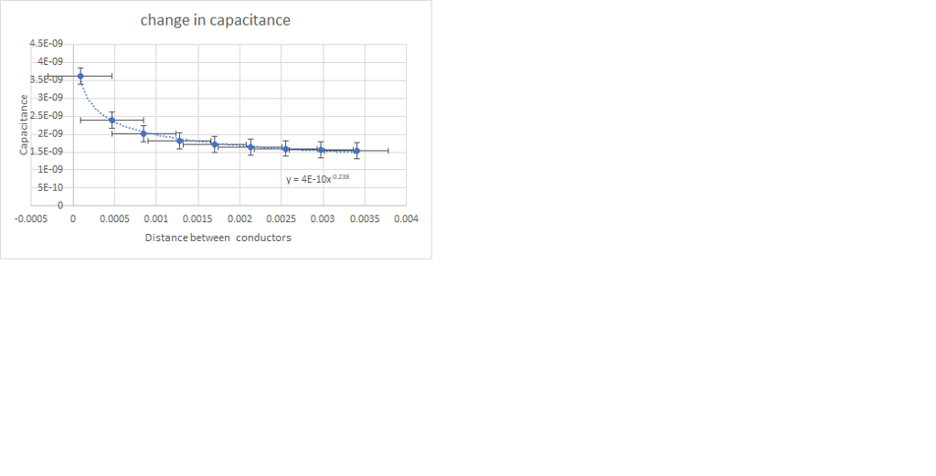
Same with this graph also thickness change in capacitance 0.000085 3.63E-09 0.0004675 2.4E-09 0.00085 2.01E-09 0.001275 1.82E-09 0.0017 1.72E-09 0.002125 1.64E-09 0.00255 1.6E-09 0.002975 1.56E-09 0.0034 1.54E-09
Here are example of the code needed distance = {0., 0.09, 0.125, 0.15, 0.17, 0.185} Enter the data for your experiments in the following cells. Note that RotTime0 refers to the case when there are zero masses attached to the wheel. RotTime1 refers to the data from when the masses are in Aperture 1, etc. rotTime0 = {} rotTime1 = {} rotTime2 = {} rotTime3 = {} rotTime4 = {} rotTime5 = {}
Let's now see how Mathematica can calculate the mean and standard deviation from a set of data. There are built-in functions to do this -- built-in functions in Mathematica start with a capital letter, and generally take some argument(s) as input(s) in a square brackets. For example, we can calculate both the mean and standard deviation of the RotTime0 data using the following two functions. Do these results agree with those you found in Excel?
Mean[rotTime0] StandardDeviation[rotTime0] We now want to create a new list that just stores the mean rotation times, and another list that stores the standard deviations. I have created the list of means, you need to create the list of standard deviations by replacing the text ?(*fill in here what you need to calculate standard deviations*)? in the input cell below with the appropriate code. meanRotTimes = {Mean[rotTime0],Mean[rotTime1], Mean[rotTime2], Mean[rotTime3], Mean[rotTime4], Mean[rotTime5]} stdDevs = {(*fill in here what you need to calculate standard deviations*)} Now of course we actually want standard uncertainties not just standard deviations, since we are using the averages as our estimates for the times. To obtain these we need to divide by , replace the text ?(*enter your n*)? below with your value of n to have Mathematica automatically divide all of the standard deviations by . meanStdDevs=stdDevs/Sqrt[(*enter your n*)] Finally, we should think about errors in the distances. Let?s set up a list called DistanceErrors. The errors on each distance were the same (0.0005 m), so we can set this list up in a slightly different way using a function called ConstantArray. The first call to this function is the value for each list element, and the second call is the number of list elements that you want to have. distanceError = ConstantArray[0.0005, 6] It is worth noting that all of the methods described in this section are just one way of getting data into Mathematica and manipulating it. There are a number of other way that are much simpler when large quantities of data are involved, and therefore do not involve manual data entry and manipulation. This method will work for our purposes though. A First Plot It is always a good idea to make sure you have entered data correctly by looking at a plot of it. This is very simple in Mathematica!
First, we must get the data into a format that Mathematica likes. Up to now, we have developed separate, one-dimensional lists for the mean rotation times and also for the distance. Mathematica would like us to create a single, two-dimensional list for our data before plotting this. So, let?s use a command called ?Thread? to put our data into a two-dimensional list -- see if you can figure out what this function is doing by evaluating it, and looking at the output. data = Thread[{distance, meanRotTimes}] ListPlot[data]
Needs["ErrorBarPlots`"] ErrorListPlot fullData=Table[{data[[i]],ErrorBar[distanceError[[i]],meanStdDevs[[i]]]},{i,1,Length[data]}] errPlot = ErrorListPlot[fullData] The above ?fullData? call creates a Table that includes both the data and the errors. Try to figure out how this is happening. Note that the ?i? is simply an index that goes from 1 to the total number of entries in ?data?, as dictated in the part of the expression: {i, 1, Length[data]}
Note that by giving the plot a name (i.e., errPlot in the above call) we can re-plot this later with more data, lines, etc. We will need this in a few sections time. Fitting the data We expect the system?s total moment of inertia to be proportional to the distance of the mass squared. Therefore, we should create these quantities.
Firstly, enter your values for the radius of the hub, the mass of the weight, and the acceleration due to gravity (remember we?re using SI units). Enter them after the equals sign, but before the semi-colon. The semi-colon simply acts to suppress the output; i.e., after you enter the values and hit shift + enter, the values will not be displayed on the next line. rHub=; mWeight =; g =; Also note that the above three variables were all defined in one ?cell?, meaning you only had to hit shift-enter once to evaluate all three variables.
The following equation calculates the total moment of inertia given the mean rotation times. Itotal = mWeight*g*rHub*(meanRotTimes)^2/(4 * Pi) - mWeight* rHub^2 linearizedData = Thread[{distance^2, Itotal}] linFit=LinearModelFit[linearizedData,x,x]; linFit["BestFitParameters"] linFit["ParameterErrors"] We can plot out nice, new linear fit with the following simple call that evaluates our linear fit between the values of 0 and 0.04 linFitPlot=Plot[linFit[x],{x,0,0.04}] linDataPlot =ListPlot[linearizedData] Show[linFitPlot,linDataPlot] linDataPlot=ListPlot[linearizedData,PlotLabel->"Linearized Data"] Add a frame, and axis labels linDataPlot=ListPlot[linearizedData,PlotLabel->"Linearized Data",Frame ->True,FrameLabel->{"Distance^2 [m^2]","Moment of Inertia [kg m^2]"}] Change the colour and shape of the points, increase the size of the labels and change the font linDataPlot=ListPlot[linearizedData,PlotLabel->"Linearized Data",Frame ->True,FrameLabel->{"Distance^2 [m^2]","Moment of Inertia [kg m^2]"},PlotStyle->Red,PlotMarkers ->{"o",15}, BaseStyle->{FontSize->15,FontFamily->Times}]; combinedPlot = Show[linDataPlot,linFitPlot]
Export["image.png",combinedPlot] Assessed Exercise Create a plot of your data that includes the full error bars, and the model fit. You will be graded on this submission according to your plot containing the following items: * Error bars in the x-direction * Error bars in the y-direction * line of best fit * labels on both axes * Title on the plot - include your name in the plot * Different colours for the line of best fit and the data * A plot legend -
Here are example of the code needed Data entry Data can be entered in Mathematica in a number of ways. The simplest is to create lists. To enter data: use a list seperated by commas and wrapped in a {}. Let's start by making a list of the radial distances that the masses were attached to the disk. Note the 'zero' distance is the case when there was no extra mass attached to the disk. Also note that we're going to work in SI units throughout. distance = {0., 0.09, 0.125, 0.15, 0.17, 0.185} Enter the data for your experiments in the following cells. Note that RotTime0 refers to the case when there are zero masses attached to the wheel. RotTime1 refers to the data from when the masses are in Aperture 1, etc. rotTime0 = {} rotTime1 = {} rotTime2 = {} rotTime3 = {} rotTime4 = {} rotTime5 = {} Let's now see how Mathematica can calculate the mean and standard deviation from a set of data. There are built-in functions to do this -- built-in functions in Mathematica start with a capital letter, and generally take some argument(s) as input(s) in a square brackets. For example, we can calculate both the mean and standard deviation of the RotTime0 data using the following two functions. Do these r
Capacitance (farad) 3E-09 2.5E-09 2E-09 1.5E-09 1E-09 5E-10 0 0 500 capacitance 1000 1/d y=5E-13x+1E-09 1500 2000 2500
Step by Step Solution
There are 3 Steps involved in it
For plotting a graph with x and y labels and a title the code is distance 2... View full answer

Get step-by-step solutions from verified subject matter experts