can u do this one

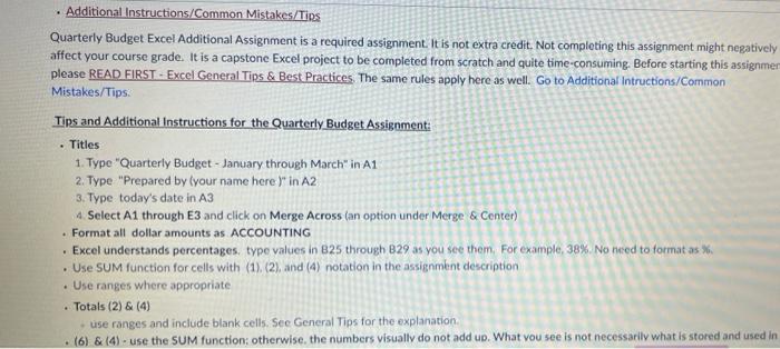
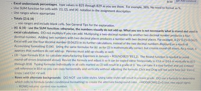
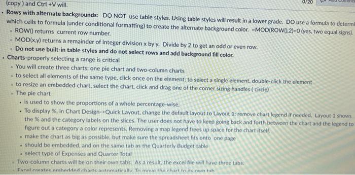
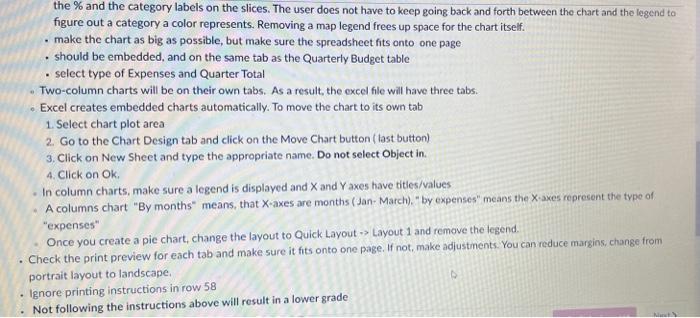
a - Additional Instructions/Common Mistakes/Tips Quarterly Budget Excel Additional Assignment is a required assignment. It is not extra credit. Not completing this assignment might negatively affect your course grade. It is a capstone Excel project to be completed from scratch and quite time-consuming. Before starting this assignmer please READ FIRST.. Excel General Tips & Best Practices. The same rules apply here as well. Go to Additional Intructions/Common Mistakes/Tips Tips and Additional Instructions for the Quarterly Budget Assignment: Titles 1. Type "Quarterly Budget - January through March" in A1 2. Type "Prepared by your name here )" in A2 3. Type today's date in A3 Select A1 through E3 and click on Merge Across (an option under Merge & Conter) Format all dollar amounts as ACCOUNTING Excel understands percentages, type values in 825 through B29 as you see them. For example, 38% No need to format as % . Use SUM function for cells with (1) (2) and (4) notation in the assignment description Use ranges where appropriate Totals (2) & (4) use ranges and include blank cells. See General Tips for the explanation . (6) & (4): use the SUM function: otherwise, the numbers visually do not add up. What you see is not necessarily what is stored and used in 0/20 # Add Comment Excel understands percentages, type values in B25 through B29 as you see them. For example, 38%. No need to format as % Use SUM function for cells with (1). (2), and (4) notation in the assignment description . Use ranges where appropriate Totals (2) & (4) use ranges and include blank cells. See General Tips for the explanation . (6) & (4) - use the SUM function; otherwise, the numbers visually do not add up. What you see is not necessarily what is stored and used in excel calculations. Do not multiply if you can add. Multiplying a two-decimal number by another two decimal number produces a four decimal number. Adding two numbers with two decimal places produces a number with two decimal places. For example, 0.250.25-0.0625, Excel will use the four decimal number (0.0625) in its further calculations, instead of the two decimal numbers displayed as a result of Accounting formatting (0.06). Using the same formulas for (6) as for (3) is mathematically correct, but creates round-off errors. As a result, it appears that numbers do not add up. Pennies must add up visually as well. (3) - type formula B14 to calculate manufacturing Expenses in January - ROUND(825*B11.2). The Round function is needed to avoid round-off errors (explained above) Revisit the formula and adjust it so it can be copied either horizontally to C14 or D14 or vertically to B15 through B18. Typing formulas individually in all cells marked as (3) will result in a grade of 0. You can take it a step further and use a mo cell reference in B14 so you can copy horizontally and vertically without adjusting the formula. Click and Drag will not work here but Ctrlto (copy) and CtrlV will Rows with alternate backgrounds: DO NOT use table styles. Using table styles will result in a lower grade. Do use a formula to determine which cells to formula (under conditional formatting) to create the alternate background color -MODIROW0,2)-0(yes, two equal signs). ROWO) returns current row number 0/20 INC . (copy) and Ctrl +V will. Rows with alternate backgrounds: DO NOT use table styles. Using table styles will result in a lower grade. Do use a formula to determi which cells to formula (under conditional formatting) to create the alternate background color. =MOD(ROW().2)-0(yes, two equal signs). ROW() returns current row number. MOD(x,y) returns a remainder of integer division x by y. Divide by 2 to get an odd or even row. Do not use built-in table styles and do not select rows and add background fill color. Charts-properly selecting a range is critical You will create three charts: one pie chart and two-column charts to select all elements of the same type, click once on the element; to select a single element, double-click the element to resize an embedded chart, select the chart, click and drag one of the corner sizing handles (circle) The pie chart is used to show the proportions of a whole percentage-wise: . To display %, in Chart Design-> Quick Layout change the default layout to Layout 1: remove chart legend if needed Layout 1 shows the % and the category labels on the slices. The user does not have to keep going back and forth between the chart and the legend to figure out a category a color represents. Removing a map legend frees up space for the chart itself make the chart as big as possible, but make sure the spreadsheet hits onto one page should be embedded, and on the same tab as the Quarterly Budget table select type of Expenses and Quarter Total Two column charts will be on their own tabs. As a result, the excel file will have three tabs Fvrolrrentes embedded harcamatically. To mua the chart to its nuntah . . the % and the category labels on the slices. The user does not have to keep going back and forth between the chart and the legend to figure out a category a color represents. Removing a map legend frees up space for the chart itself. make the chart as big as possible, but make sure the spreadsheet fits onto one page should be embedded, and on the same tab as the Quarterly Budget table select type of Expenses and Quarter Total Two-column charts will be on their own tabs. As a result, the excel file will have three tabs. Excel creates embedded charts automatically. To move the chart to its own tab 1. Select chart plot area 2. Go to the Chart Design tab and click on the Move Chart button ( tast button) 3. Click on New Sheet and type the appropriate name. Do not select Object in 4. Click on Ok In column charts, make sure a legend is displayed and X and Yaxes have titles/values A columns chart "By months means that X-axes are months (Jan-March)" by expenses" means the X-axes represent the type of "expenses" Once you create a pie chart, change the layout to Quick Layout -> Layout 1 and remove the legend. Check the print preview for each tab and make sure it fits onto one page. If not, make adjustments. You can reduce margins, change from portrait layout to landscape. Ignore printing instructions in row 58 Not following the instructions above will result in a lower grade