Can you please help me answer Part B, C, & D? How do I change the formulas for the difference in monthly payments?

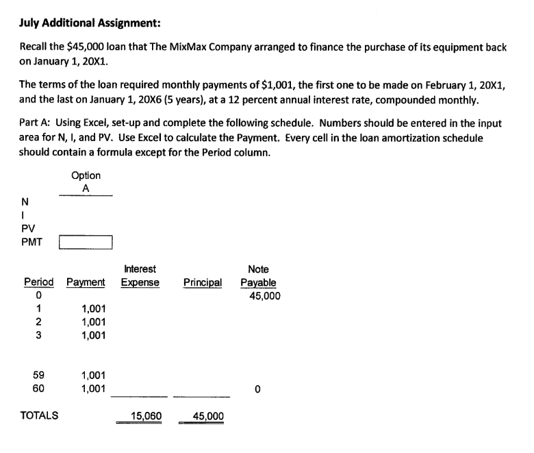
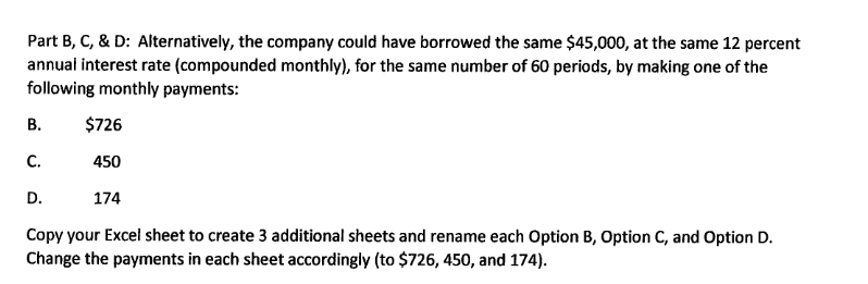
July Additional Assignment: Recall the $45,000 loan that The MixMax Company arranged to finance the purchase of its equipment back on January 1, 20X1. The terms of the loan required monthly payments of $1,001, the first one to be made on February 1, 20x1, and the last on January 1, 20X6 (5 years), at a 12 percent annual interest rate, compounded monthly. Part A: Using Excel, set-up and complete the following schedule. Numbers should be entered in the input area for N, I, and PV. Use Excel to calculate the payment. Every cell in the loan amortization schedule should contain a formula except for the Period column. Option N 1 PV PMT Interest Expense Principal Note Payable 45,000 Period Payment 0 1 1,001 2 1,001 3 1,001 59 60 1,001 1,001 0 TOTALS 15,060 45,000 Part B, C, & D: Alternatively, the company could have borrowed the same $45,000, at the same 12 percent annual interest rate (compounded monthly), for the same number of 60 periods, by making one of the following monthly payments: B. $726 C. 450 D. 174 Copy your Excel sheet to create 3 additional sheets and rename each Option B, Option C, and Option D. Change the payments in each sheet accordingly (to $726, 450, and 174). July Additional Assignment: Recall the $45,000 loan that The MixMax Company arranged to finance the purchase of its equipment back on January 1, 20X1. The terms of the loan required monthly payments of $1,001, the first one to be made on February 1, 20x1, and the last on January 1, 20X6 (5 years), at a 12 percent annual interest rate, compounded monthly. Part A: Using Excel, set-up and complete the following schedule. Numbers should be entered in the input area for N, I, and PV. Use Excel to calculate the payment. Every cell in the loan amortization schedule should contain a formula except for the Period column. Option N 1 PV PMT Interest Expense Principal Note Payable 45,000 Period Payment 0 1 1,001 2 1,001 3 1,001 59 60 1,001 1,001 0 TOTALS 15,060 45,000 Part B, C, & D: Alternatively, the company could have borrowed the same $45,000, at the same 12 percent annual interest rate (compounded monthly), for the same number of 60 periods, by making one of the following monthly payments: B. $726 C. 450 D. 174 Copy your Excel sheet to create 3 additional sheets and rename each Option B, Option C, and Option D. Change the payments in each sheet accordingly (to $726, 450, and 174)