case study

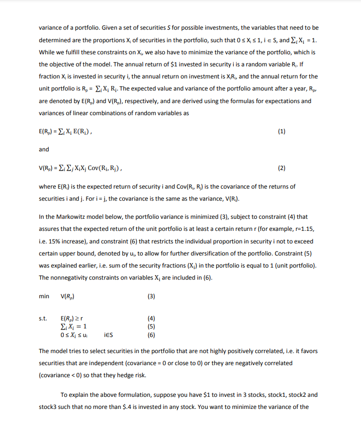
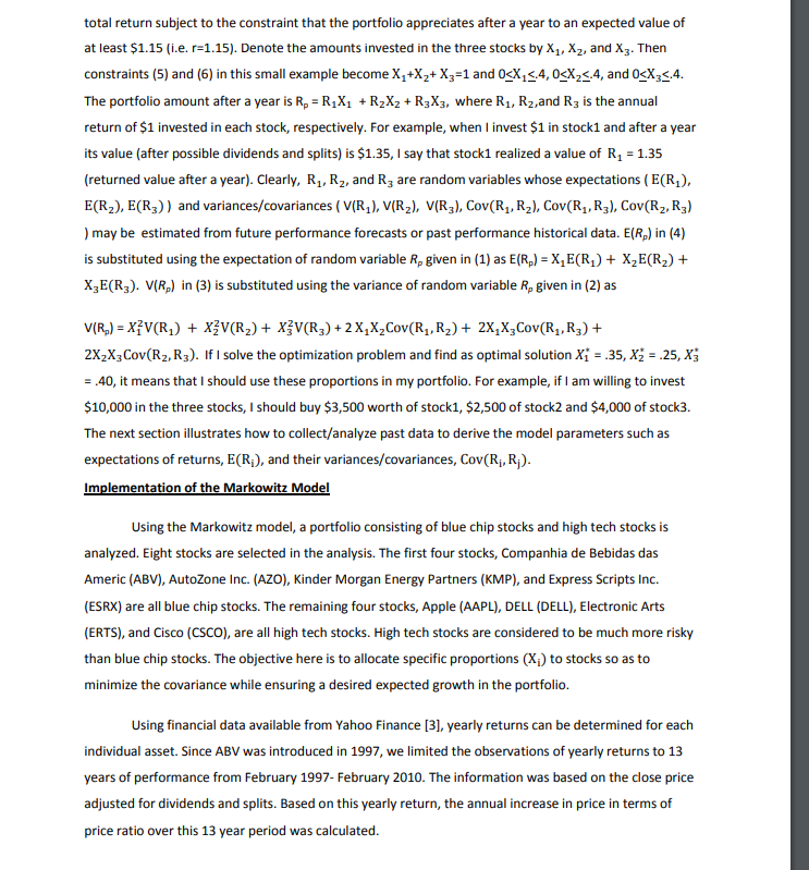
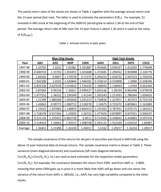
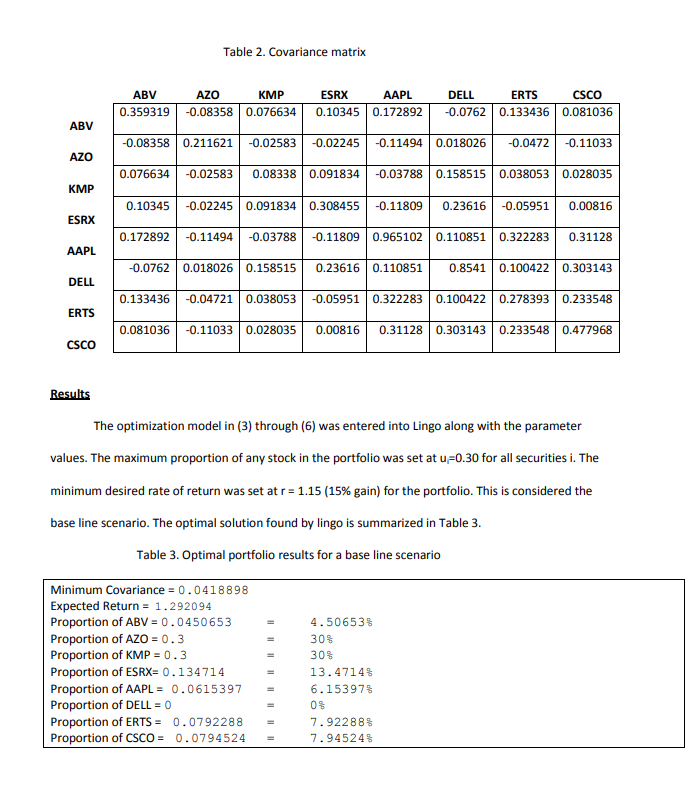
2. Briefly, in a few sentences (avoid symbols and equations as much as possible), describe the mathematical model developed in this paper. In particular, what is the objective, decision variables, types of constraints in the model, and data required. 3. Looking at the optimal portfolio found in Table 3, which stock(s) did not make it? How is the projected expected return compared to the minimum specified (15%) gain? What is the surplus of Constraint 4? Background Portfolio models use two criteria to evaluate investments: expected return and risk. The investor wants the former to be high and the latter to be low. Risks can be measured in many ways. In this case study, the measure we would be using is the variance in return. The portfolio with the highest rate of return is not necessary the one with the least variability. A portfolio with an extremely high return may be subjected to an unacceptable high degree of variability and therefore, down risk. The proper choice among portfolios depends on the willingness of an investor to assume risk. In other words, it depends on the risk profile of the investor: the investor can be risk averse, risk neutral, or risk seeking. Very often, there is a trade-off between risk and rate of return. This case study explores this trade off and minimizes the risk of the portfolio while allowing the investor to still be able to achieve his/her desired expected rate of return. Specifically, we will discuss how to use the Markowitz Model in selecting a portfolio. Markowitz Portfolio Selection Harry M. Markowitz introduced the portfolio model in the March 1952 issue of Journal of Finance titled Portfolio Selection. In this model, he assumes that an investor has two considerations when constructing an investment portfolio: expected return and variance in return, i.e. risk [1,2]. Variance measures the variability in realized return around the expected return and this volatility is a measure of the risk. The higher the variance, the riskier is the investment. The model requires two inputs: (1) the estimated expected annual return for each investment and (2) the covariance matrix of returns. The covariance matrix characterizes the variability of each individual investment (variances contained in the main diagonal elements) and also how one investment fluctuates compared to another (covariances contained in the upper or lower diagonal elements - symmetric matrix). High positive covariance between two securities indicates that a decrease in one security's return is likely to correspond to a decrease in the other (hence riskier) as there is less hedging. A covariance close to zero means the investments have relatively independent return rates. A negative covariance means a decrease in one security's return is likely to correspond to an increase in the other and vice versa. This case study demonstrates how to reduce the risk of asset portfolios by selecting assets (e.g. securities, such as stocks and bonds) whose values are not highly correlated. This has come to be known as diversification of assets. The Markowitz model deals mainly with the statistic that describes the variance of a portfolio. Given a set of securities for possible investments, the variables that need to be determined are the proportions X of securities in the portfolio, such that 0sX 51, i e S, and X;X; = 1. While we fulfill these constraints on X, we also have to minimize the variance of the portfolio, which is the objective of the model. The annual return of $1 invested in security i is a random variable R. If fraction X, is invested in security i, the annual return on investment is XR, and the annual return for the unit portfolio is R2 = 2;X; R. The expected value and variance of the portfolio amount after a year, Rp are denoted by E(R) and V(R), respectively, and are derived using the formulas for expectations and variances of linear combinations of random variables as E(R.) = XXE(R) (1) and V(R.) = :;X;X; Cov(Ri, R), (2) where E(R) is the expected return of security i and Cov(Ri, R) is the covariance of the returns of securities i and j. For i = j, the covariance is the same as the variance, V(R.). In the Markowitz model below, the portfolio variance is minimized (3), subject to constraint (4) that assures that the expected return of the unit portfolio is at least a certain return r (for example, r=1.15, i.e. 15% increase), and constraint (6) that restricts the individual proportion in security i not to exceed certain upper bound, denoted by U, to allow for further diversification of the portfolio. Constraint (5) was explained earlier, i.e. sum of the security fractions (X) in the portfolio is equal to 1 (unit portfolio). The nonnegativity constraints on variables X; are included in (6). min V(R) (3) s.t. E(R) 2r = 1 Os Xi su (4) (5) (6) IES The model tries to select securities in the portfolio that are not highly positively correlated, i.e. it favors securities that are independent (covariance = 0 or close to 0) or they are negatively correlated (covariance