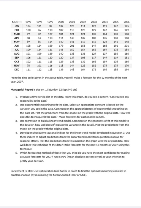
Case Study 2: Forecasting Box Office Returns For years, people in the motion picture industry-critics, film historians, and others - have eagerly awaited the second issue in January of Variety. Long considered the show business bible, Variety is a weekly trade newspaper that reports on all aspects of the entertainment industry, movies, television, recordings, concert tours, and so on. The second issue in January, called the Anniversary Edition, summarizes how the entertainment industry fared in the previous year, both artistically and commercially In this issue, Variety publishes its list of All Time Film Rental Champs. This list indicates, in descending order, motion pictures and the amount of money they returned to the studio. Because a movie theater rents a film from a studio for a limited time, the money paid for admission by ticket buyers is split between the studio and theater owner. For example, if a ticket buyer pays $12 to see a particular movie, the theater owner keeps about $6 and the studio receives the other $6. The longer a movie plays in a theater, the greater the percentage of the admission price returned to the studio. A film playing for an entire summer could eventually return as much as 90% of the $12 to the studio. The theater owner also benefits from such a success because although the owner's percentage of the admission price is small, the sales of concessions (candy, soda and so on) provide greater profits. Thus, both the studio and the theater owner win when a film continues to draw audiences for a long time. Variety lists the rental figures (the actual dollar amounts returned to the studios) that the films have accrued in their domestic releases (United States and Canada). In addition, Variety provides a monthly Box-Office Barometer of the film industry, which is a profile of the month's domestic box-office returns. This profile is not measured in dollars, but scaled according to some standard. By the late 1980's, for example, the scale was based on numbers around 100, with 100 representing the average box-office return of 1990. The figures from 1997 to 2006 are given in the table below and in the file BoxOffice.xlsx in blackboard. All the figures are scaled around the 1990's box-office returns, but instead of dollars, artificial numbers are used. Film executives can get a relative indication of the box-office figures compared to the arbitrary 1990 scale. For example, in January 1997 the box-office returns to the film industry were 95% of the average that year, whereas in January 1998 the returns were 104% of the average of 1990 (or, they were 4% above the average of 1990's figure). 2002 2001 125 118 121 111 123 2003 127 129 132 108 2004 119 147 164 121 1999 8B 110 129 113 114 169 131 140 139 MONTH JAN FEB MAR APR MAY JUN JUL AUG SEP OCT NOV DEC 135 1997 104 100 99 88 89 108 109 101 106 102 78 111 115 1998 101 96 82 84 85 124 134 109 121 111 101 112 2006 145 149 148 148 148 201 184 2000 132 109 101 111 140 179 145 140 120 129 118 139 141 201 152 119 156 154 136 105 132 2005 147 146 133 148 141 191 178 156 119 138 175 139 138 166 124 168 159 137 149 159 175 195 120 115 116 128 149 155 129 117 166 152 173 137 138 144 151 166 170 194 123 148 164 188 From the time series given in the above table, you will make a forecast for the 12 months of the next year, 2007. Managerial Report is due on ... Saturday, 12 Sept (40 pts) 1. Produce a time series plot of the data. From this graph, do you see a pattern? Can you see any seasonality in the data? 2. Use exponential smoothing to fit the data. Select an appropriate constant a based on the variation you see in the data. Comment on the appropriateness of exponential smoothing on this data set. Plot the predictions from this model on the graph with the original data. How well does this technique fit the data? Make forecasts for each month in 2007. 3. Use regression to build a linear trend model. Comment on the goodness-of-fit of this model to the data for, how well does R explain the variance in the data?). Plot the predictions from this model on the graph with the original data. 4. Develop multiplicative seasonal indices for the linear trend model developed in question 3. Use these indices to adjust predictions from the linear trend model from question 3 above for seasonal effects. Plot the predictions from this model on the graph with the original data. How well does this technique fit the data? Make forecasts for the next 12 months of 2007 using this technique 5. Which forecasting method of those that you tried do you have the most confidence for making accurate forecasts for 2007? Use MAPE (mean absolute percent error) as your criterion to justify your decision. Enrichment (5 pts): Use Optimization (and Solver in Exce) to find the optimal smoothing constant in problem 2 above (by minimizing the Mean Squared Error or MSE). Case Study 2: Forecasting Box Office Returns For years, people in the motion picture industry-critics, film historians, and others - have eagerly awaited the second issue in January of Variety. Long considered the show business bible, Variety is a weekly trade newspaper that reports on all aspects of the entertainment industry, movies, television, recordings, concert tours, and so on. The second issue in January, called the Anniversary Edition, summarizes how the entertainment industry fared in the previous year, both artistically and commercially In this issue, Variety publishes its list of All Time Film Rental Champs. This list indicates, in descending order, motion pictures and the amount of money they returned to the studio. Because a movie theater rents a film from a studio for a limited time, the money paid for admission by ticket buyers is split between the studio and theater owner. For example, if a ticket buyer pays $12 to see a particular movie, the theater owner keeps about $6 and the studio receives the other $6. The longer a movie plays in a theater, the greater the percentage of the admission price returned to the studio. A film playing for an entire summer could eventually return as much as 90% of the $12 to the studio. The theater owner also benefits from such a success because although the owner's percentage of the admission price is small, the sales of concessions (candy, soda and so on) provide greater profits. Thus, both the studio and the theater owner win when a film continues to draw audiences for a long time. Variety lists the rental figures (the actual dollar amounts returned to the studios) that the films have accrued in their domestic releases (United States and Canada). In addition, Variety provides a monthly Box-Office Barometer of the film industry, which is a profile of the month's domestic box-office returns. This profile is not measured in dollars, but scaled according to some standard. By the late 1980's, for example, the scale was based on numbers around 100, with 100 representing the average box-office return of 1990. The figures from 1997 to 2006 are given in the table below and in the file BoxOffice.xlsx in blackboard. All the figures are scaled around the 1990's box-office returns, but instead of dollars, artificial numbers are used. Film executives can get a relative indication of the box-office figures compared to the arbitrary 1990 scale. For example, in January 1997 the box-office returns to the film industry were 95% of the average that year, whereas in January 1998 the returns were 104% of the average of 1990 (or, they were 4% above the average of 1990's figure). 2002 2001 125 118 121 111 123 2003 127 129 132 108 2004 119 147 164 121 1999 8B 110 129 113 114 169 131 140 139 MONTH JAN FEB MAR APR MAY JUN JUL AUG SEP OCT NOV DEC 135 1997 104 100 99 88 89 108 109 101 106 102 78 111 115 1998 101 96 82 84 85 124 134 109 121 111 101 112 2006 145 149 148 148 148 201 184 2000 132 109 101 111 140 179 145 140 120 129 118 139 141 201 152 119 156 154 136 105 132 2005 147 146 133 148 141 191 178 156 119 138 175 139 138 166 124 168 159 137 149 159 175 195 120 115 116 128 149 155 129 117 166 152 173 137 138 144 151 166 170 194 123 148 164 188 From the time series given in the above table, you will make a forecast for the 12 months of the next year, 2007. Managerial Report is due on ... Saturday, 12 Sept (40 pts) 1. Produce a time series plot of the data. From this graph, do you see a pattern? Can you see any seasonality in the data? 2. Use exponential smoothing to fit the data. Select an appropriate constant a based on the variation you see in the data. Comment on the appropriateness of exponential smoothing on this data set. Plot the predictions from this model on the graph with the original data. How well does this technique fit the data? Make forecasts for each month in 2007. 3. Use regression to build a linear trend model. Comment on the goodness-of-fit of this model to the data for, how well does R explain the variance in the data?). Plot the predictions from this model on the graph with the original data. 4. Develop multiplicative seasonal indices for the linear trend model developed in question 3. Use these indices to adjust predictions from the linear trend model from question 3 above for seasonal effects. Plot the predictions from this model on the graph with the original data. How well does this technique fit the data? Make forecasts for the next 12 months of 2007 using this technique 5. Which forecasting method of those that you tried do you have the most confidence for making accurate forecasts for 2007? Use MAPE (mean absolute percent error) as your criterion to justify your decision. Enrichment (5 pts): Use Optimization (and Solver in Exce) to find the optimal smoothing constant in problem 2 above (by minimizing the Mean Squared Error or MSE)