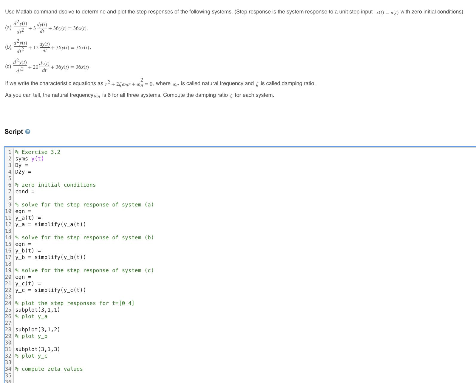
Use Matlab command dsolve to determine and plot the step responses of the following systems. (Step response is the system response to a unit step input x(t) = u(t) with zero initial conditions). dy(t) (a) d1 +3 +36y(t) = 36x(t), dy(t) dt (b) + 12 dy(t) + 36y(t) = 36x(t), dy(t) dt2 d y(t) (c) + 20 dy(t) + 36y(t) = 36x(t). d12 dt 2 If we write the characteristic equations as r +25@nr + n = 0, where an is called natural frequency and is called damping ratio. As you can tell, the natural frequency on is 6 for all three systems. Compute the damping ratio for each system. Script> 1% Exercise 3.2 2 syms y(t) 3 Dy = 4 D2y = 6% zero initial conditions 7 cond= 9% solve for the step response of system (a) 10 eqn = 11 y_a(t) = 12 y_a= simplify (y_a(t)) 13 14 % solve for the step response of system (b) 15 eqn = 16 y_b(t) = 17 y_b = simplify(y_b(t)) 18 19% solve for the step response of system (c) 20 eqn = 21 y_c(t) = 22 y_c= simplify (y_c(t)) 23 24 % plot the step responses for t= [04] 25 subplot (3,1,1) 26% plot y_a 27 28 subplot(3,1,2) 29 % plot y_b 30 31 subplot (3,1,3) 32 % plot y_c 33 34 % compute zeta values 35 36