comment, thanks

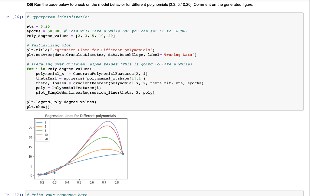
Q5) Run the code below to check on the model behavior for different polynomials (2,3,5,10,20). Comment on the generated figure. In [26]: * Hyperparam initialization eta = 0.25 epochs = 500000 # This will take a while but you can set it to 10000. Poly_degree_values = [2, 3, 5, 10, 20] # Initializing plot plt.title("Regression Lines for Different polynomials") plt.scatter(data. GranulesDiameter, data. Beachslope, label='Traning Data') # iterating over different alpha values (This is going to take a while) for i in Poly_degree_values: polynomial_x = GeneratePolynomialFeatures (X, i) thetaInit np.zeros((polynomial_x.shape[1],1)) theta, losses = gradientDescent (polynomial_x, y, thetaInit, eta, epochs) poly - PolynomialFeatures(i) plot_SimpleNonlinearRegression_line (theta, x, poly) plt.legend (Poly_degree_values) plt.show() Regression Lines for Different polynomials 2 25 5 20 10 20 15 10 5 0 02 03 04 0.5 0.6 0.7 0.8 In 1271; # Write your response here