COMPLETE THE FOLLOWING USING THE ATTACHED DOCUMENTS

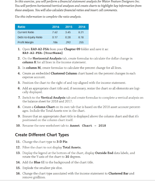
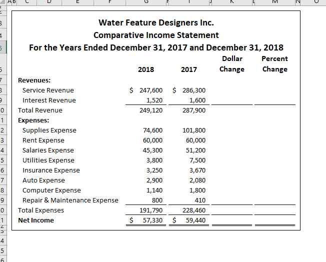
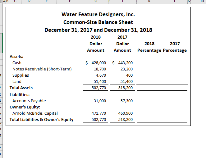
In this exercise, you will perform a financial statement analysis for Water Feature Designers Inc. You will perform horizontal/vertical analyses and create charts to highlight key information from these analyses. You will also calculate financial ratios and insert cell comments. Use this information to complete the ratio analysis. Ratio Current Ratio Debt-to-Equity Ratio Profit Margin 2016 7.62 0.17 .186 2015 3.45 0.28 292 2014 8.21 0.18 255 1. Open EA9-A2-FSA from your Chapter 09 folder and save it as: EA9-A2-FSA-[YourName] 2. On the Horizontal Analysis tab, create formulas to calculate the dollar change in column K for all lines in the income statement. 3. In column M. create formulas to calculate the percent change for all lines. 4. Create an embedded Clustered Column chart based on the percent changes in each expense account. 5. Position the chart to the right of and top-aligned with the income statement 6. Add an appropriate chart title and, if necessary, resize the chart so all elements are logi cally displayed. 7. Switch to the Vertical Analysis tab and create formulas to complete a vertical analysis on the balance sheet for 2018 and 2017. 8. Create a Column Chart on its own tab that is based on the 2018 asset account percent- ages. Include the Total Assets row in the chart. 9. Ensure that an appropriate chart title is displayed above the column chart and that it's positioned on the column chart itself. 10. Rename the new worksheet tab to: Asset Chart - 2018 Create Different Chart Types 11. Change the chart type to 3-D Pie. 12. Filter the chart to not display Total Assets. 13. Display the legend at the bottom of the chart, display Outside End data labels, and rotate the Y-axis of the chart to 30 degrees. 14. Add the Blue fill to the background of the chart title. 15. Explode the smallest pie slice. 16. Change the chart type associated with the income statement to Clustered Bar and remove gridlines. Apply Chart Layouts, Chart Styles, and Sparklines 17. Apply Layout 6 and Style 7 to the 3-D Pie chart. 18. Use filters to remove Land from the 3-D Pie chart. 19. Adjust the data labels to display as Percentages with 2 decimal places. 20. Display Column Sparklines to the right of each asset, liability, and owner's equity account in the balance sheet. 21. Adjust the borders and the balance sheet to include the sparklines. 22. Insert a Sparkline Trends header in the appropriate location, making sure its formatting is consistent with that of the adjacent cell entries. Calculate Ratios and Insert Cell Comments 23. Create a new worksheet named: Financial Ratios 24. Enter headers for the five-year period from 2014-2018 in the range B1:F1, starting with the most recent year. 25. In order, enter these headings in the range A2:A4: Current Ratio, Debt-to- Equity Ratio, and Profit Margin 26. Format all headers with bold formatting, add a bottom border and center alignment to all year headers, and expand the width of column A to 20. 27. Create formulas to calculate the ratios for 2018 and 2017 28. Enter the ratios for 2016, 2015, and 2014 based on the table in the instructions. 29. Apply Comma Style to all current and debt-to-equity ratios and apply Percent Style with one decimal place to all profit margins. 30. Insert Line Sparklines to the right of each set of ratios, displaying all five years of ratio data. 31. Insert comments in the cells for the largest profit margin and smallest debt-to-equity ratio to indicate that these require further investigation 32. Display all comments in the worksheet. 33. Enter a response in the comment for the largest profit margin, indicating that a single large client led to inflated earnings for the year. Make sure the response is distinct from the original comment. 34. If necessary, resize the profit margin cell comment so it is entirely visible. 35. Embed a Line chart below the ratio data that displays the trend in the current ratio over the five-year period. 36. Modify the chart to include a chart title. 37. Save and close the file. AB C D E F G K L M NU m ch Water Feature Designers Inc. Comparative Income Statement For the Years Ended December 31, 2017 and December 31, 2018 Dollar Percent 2018 2017 Change Change Revenues: Service Revenue $ 247,600 $ 286,300 Interest Revenue 1,520 1,600 Total Revenue 249,120 287,900 Expenses: Supplies Expense 74,600 101,800 Rent Expense 60,000 60,000 Salaries Expense 45,300 51,200 Utilities Expense 3,800 7,500 Insurance Expense 3,250 3,670 Auto Expense 2,900 2,080 Computer Expense 1,140 1,800 Repair & Maintenance Expense 800 410 Total Expenses 191,790 228,460 Net Income $ 57,330 $ 59,440 in o o o o - in ABLV MN Water Feature Designers, Inc. Common-Size Balance Sheet December 31, 2017 and December 31, 2018 2018 2017 Dollar D ollar 2018 2017 Amount Amount Percentage Percentage Assets: Cash $ 428,000 $443,200 Notes Receivable (Short-Term) 18,700 23,200 Supplies 4,670 400 Land 51,400 51,400 Total Assets 502,770 518,200 Liabilities: Accounts Payable 31,000 57,300 Owner's Equity: Arnold McBride, Capital 471,770 460,900 Total Liabilities & Owner's Equity 502,770 518,200