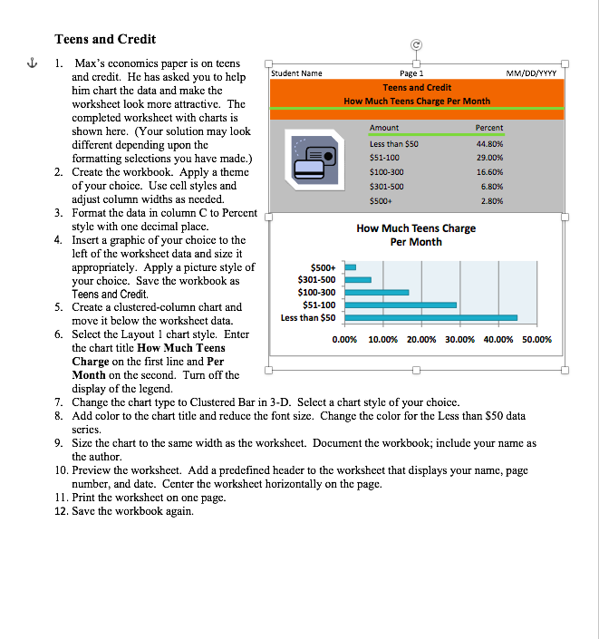
completed worksheet with charts is shown here. (Your solution may look different depending upon the formatting selections you have made.) 2. Create the workbook. Apply a theme of your choice. Use cell styles and adjust column widths as needed. 3. Format the data in column C to Percent style with one decimal place. 4. Insert a graphic of your choice to the left of the worksheet data and size it appropriately. Apply a picture style of your choice. Save the workbook as Teens and Credit. 5. Create a clustered-column chart and move it below the worksheet data. 6. Select the Layout 1 chart style. Enter the chart title How Much Teens Charge on the first line and Per Month on the second. Turn off the display of the legend. 7. Change the chart type to Clustered Bar in 3-D. Select a chart style of your choice. 8. Add color to the chart title and reduce the font size. Change the color for the Less than $50 data series. 9. Size the chart to the same width as the worksheet. Document the workbook; include your name as the author. 10. Preview the worksheet. Add a predefined header to the worksheet that displays your name, page number, and date. Center the worksheet horizontally on the page. 11. Print the worksheet on one page. 12. Save the workbook again. completed worksheet with charts is shown here. (Your solution may look different depending upon the formatting selections you have made.) 2. Create the workbook. Apply a theme of your choice. Use cell styles and adjust column widths as needed. 3. Format the data in column C to Percent style with one decimal place. 4. Insert a graphic of your choice to the left of the worksheet data and size it appropriately. Apply a picture style of your choice. Save the workbook as Teens and Credit. 5. Create a clustered-column chart and move it below the worksheet data. 6. Select the Layout 1 chart style. Enter the chart title How Much Teens Charge on the first line and Per Month on the second. Turn off the display of the legend. 7. Change the chart type to Clustered Bar in 3-D. Select a chart style of your choice. 8. Add color to the chart title and reduce the font size. Change the color for the Less than $50 data series. 9. Size the chart to the same width as the worksheet. Document the workbook; include your name as the author. 10. Preview the worksheet. Add a predefined header to the worksheet that displays your name, page number, and date. Center the worksheet horizontally on the page. 11. Print the worksheet on one page. 12. Save the workbook again