Consider EOQ model with planned backorders. Suppose that unlike the model assumption, each unit of backlogged inventory incurs a one time penalty cost of d regardless of the length of the backlog. You still have to satisfy the demand fully in each cycle. Write the total cost function per cycle. Write the cost function per unit of time. Derive the the conditions (based on the parameters of the model) under which at same cycle time the model with backlog cost not proportional to time incurs a higher backlog (not cost) than the model with backlog cost proportional to time. Explain the result in English.

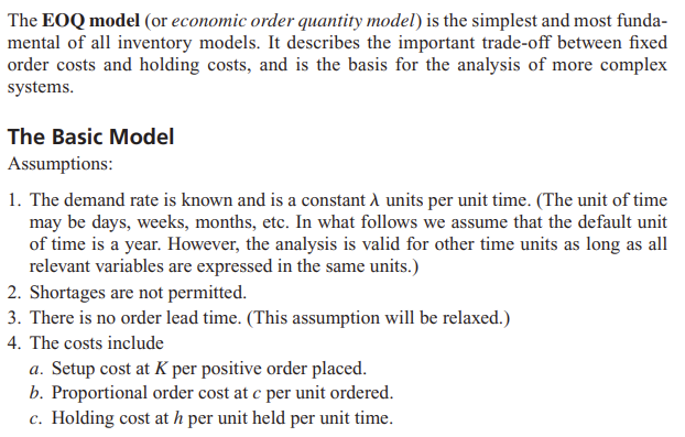
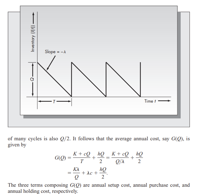
The EOQ model (or economic order quantity model) is the simplest and most funda- mental of all inventory models. It describes the important trade-off between fixed order costs and holding costs, and is the basis for the analysis of more complex systems. The Basic Model Assumptions: 1. The demand rate is known and is a constant , units per unit time. (The unit of time may be days, weeks, months, etc. In what follows we assume that the default unit of time is a year. However, the analysis is valid for other time units as long as all relevant variables are expressed in the same units.) 2. Shortages are not permitted. 3. There is no order lead time. (This assumption will be relaxed.) 4. The costs include a. Setup cost at K per positive order placed. b. Proportional order cost at c per unit ordered. c. Holding cost at h per unit held per unit time. Inventory (1) - Slope = -1 Timet + + of many cycles is also Q/2. It follows that the average annual cost, say G(Q), is given by K + cQ hQK+cQhQ GO) 2 Q1 2 hQ +ac+ Q 2 The three terms composing GQ) are annual setup cost, annual purchase cost, and annual holding cost, respectively. The EOQ model (or economic order quantity model) is the simplest and most funda- mental of all inventory models. It describes the important trade-off between fixed order costs and holding costs, and is the basis for the analysis of more complex systems. The Basic Model Assumptions: 1. The demand rate is known and is a constant , units per unit time. (The unit of time may be days, weeks, months, etc. In what follows we assume that the default unit of time is a year. However, the analysis is valid for other time units as long as all relevant variables are expressed in the same units.) 2. Shortages are not permitted. 3. There is no order lead time. (This assumption will be relaxed.) 4. The costs include a. Setup cost at K per positive order placed. b. Proportional order cost at c per unit ordered. c. Holding cost at h per unit held per unit time. Inventory (1) - Slope = -1 Timet + + of many cycles is also Q/2. It follows that the average annual cost, say G(Q), is given by K + cQ hQK+cQhQ GO) 2 Q1 2 hQ +ac+ Q 2 The three terms composing GQ) are annual setup cost, annual purchase cost, and annual holding cost, respectively