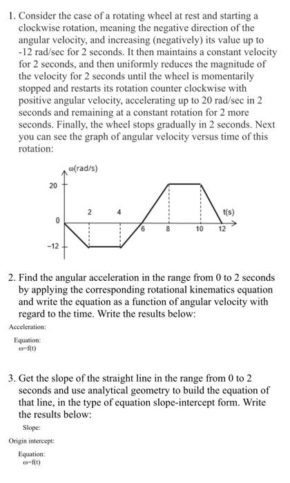
1. Consider the case of a rotating wheel at rest and starting a clockwise rotation, meaning...

 

  

  

 

   

Transcribed Image Text:

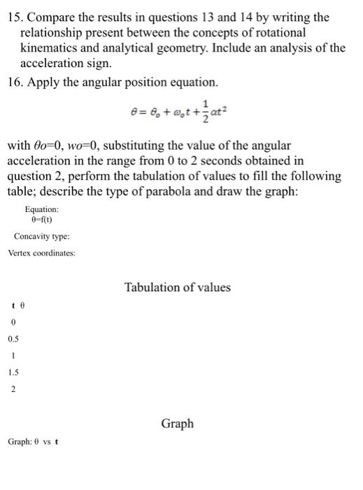
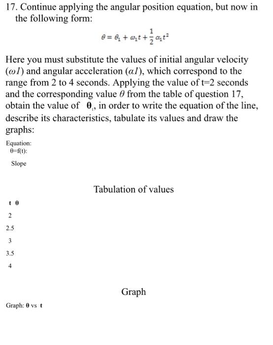
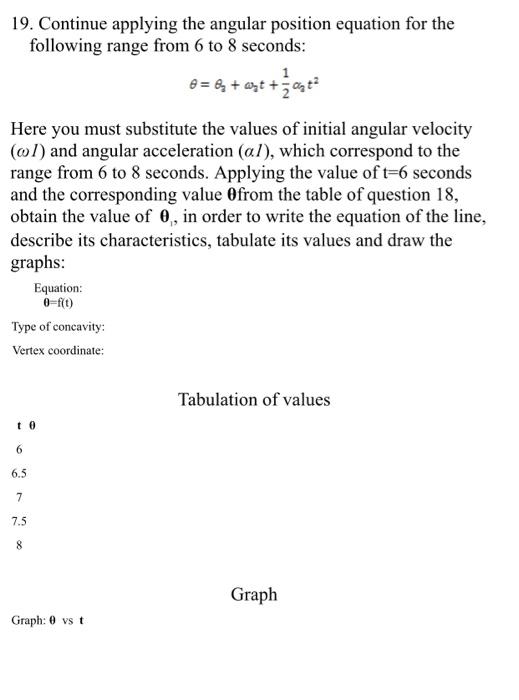
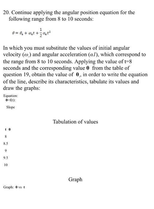
1. Consider the case of a rotating wheel at rest and starting a clockwise rotation, meaning the negative direction of the angular velocity, and increasing (negatively) its value up to -12 rad/sec for 2 seconds. It then maintains a constant velocity for 2 seconds, and then uniformly reduces the magnitude of the velocity for 2 seconds until the wheel is momentarily stopped and restarts its rotation counter clockwise with positive angular velocity, accelerating up to 20 rad/sec in 2 seconds and remaining at a constant rotation for 2 more seconds. Finally, the wheel stops gradually in 2 seconds. Next you can see the graph of angular velocity versus time of this rotation: Equation: co=f(t) 20 0 Equation: co-f(t) -12 (rad/s) 2 6 t(s) 2. Find the angular acceleration in the range from 0 to 2 seconds by applying the corresponding rotational kinematics equation and write the equation as a function of angular velocity with regard to the time. Write the results below: Acceleration: 10 12 3. Get the slope of the straight line in the range from 0 to 2 seconds and use analytical geometry to build the equation of that line, in the type of equation slope-intercept form. Write the results below: Slope: Origin intercept: 5. Determine how is the acceleration in the range from 2 to 4 seconds where the velocity is constant. Also determine the slope of the straight line and the slope-intercept equation, writing the results below: Acceleration: Slope: Origin intercept: Equation: (0=f(1) 6. Find the angular acceleration in the range from 4 to 6 seconds by applying the corresponding rotational kinematics equation and write the equation as a function of angular velocity with regard to the time. Write the results below: Acceleration: Equation: o-f(t) 7. Get the slope of the straight line in the range from 4 to 6 seconds and use analytical geometry to build the equation of that line, in the slope-intercept equation form. Write the results below: Slope: Origin intercept: Equation: co-f(t) 8. Compare the results in questions 6 and 7 by writing the relationship between the concepts of rotational kinematics and analytical geometry. Include an analysis of the acceleration sign. 9. Find the angular acceleration in the range from 6 to 8 seconds by applying the corresponding rotational kinematics equation and write the equation as a function of angular velocity with regard to the time. Write the results below: Acceleration: Equation: o-f(t) 10. Get the slope of the straight line in the range from 6 to 8 seconds and use analytical geometry to build the equation of that line, in the type of equation slope-intercept form. Write the results below: Slope: Origin intercept: Equation: 0-f(t) 11. Compare the results in questions 9 and 10 by writing the relationship between the concepts of rotational kinematics and analytical geometry. Include an analysis of the acceleration sign. 12. Determine how is the acceleration in the range from 8 to 10 seconds where the velocity is constant. Also, determine the slope of the straight line and the slope-intercept equation; write the results below: Acceleration: Slope: Origin intercept: Equation: co=f(t) 13. Find the angular acceleration in the range from 10 to 12 seconds by applying the corresponding rotational kinematics equation and write the equation as a function of angular velocity with respect to time. Write the results below: Acceleration: Equation: o-f(t) 14. Get the slope of the straight line in the range from 10 to 12 seconds and use analytical geometry to build the equation of that line, in the slope-intercept form. Write the results below: Slope: Origin intercept: Equation: to-f(t) 15. Compare the results in questions 13 and 14 by writing the relationship present between the concepts of rotational kinematics and analytical geometry. Include an analysis of the acceleration sign. 16. Apply the angular position equation. 8= o+wot+ 1/2 at ² with 00-0, wo-0, substituting the value of the angular acceleration in the range from 0 to 2 seconds obtained in question 2, perform the tabulation of values to fill the following table; describe the type of parabola and draw the graph: Equation: 0=f(t) Concavity type: Vertex coordinates: te 0 0.5 I 1.5 2 Graph: 0 vs t Tabulation of values Graph 17. Continue applying the angular position equation, but now in the following form: 0 = 0₁ +₁ +2₂² Here you must substitute the values of initial angular velocity (1) and angular acceleration (al), which correspond to the range from 2 to 4 seconds. Applying the value of t=2 seconds and the corresponding value from the table of question 17, obtain the value of 0, in order to write the equation of the line, describe its characteristics, tabulate its values and draw the graphs: Equation: 0=f(t): Slope te 2 2.5 3 3.5 4 Graph: 0 vs t Tabulation of values Graph 18. Continue applying the angular position equation for the following range from 4 to 6 seconds: Here you must substitute the values of initial angular velocity (1) and angular acceleration (al) which correspond to the range from 4 to 6 seconds. Applying the value of t=4 seconds and the corresponding value Ofrom the table of question 18, obtain the value of 0₁, in order to write the equation of the line, describe its characteristics, tabulate its values and draw the graphs: Equation: 0-f(t) Type of concavity: Vertex coordinates: t0 4.5 5 5.5 6 1 0 = 8₂ + ₂t + 2 α₂t² Graph: 0 vs t Tabulation of values Graph 19. Continue applying the angular position equation for the following range from 6 to 8 seconds: 0 = 8₂ + ₂t + a₂² Here you must substitute the values of initial angular velocity (@I) and angular acceleration (a1), which correspond to the range from 6 to 8 seconds. Applying the value of t-6 seconds and the corresponding value Ofrom the table of question 18, obtain the value of 0₁, in order to write the equation of the line, describe its characteristics, tabulate its values and draw the graphs: Type of concavity: Vertex coordinate: Equation: 0-f(t) t0 6 6.5 7 7.5 8 Graph: 0 vs t Tabulation of values Graph 20. Continue applying the angular position equation for the following range from 8 to 10 seconds: 0 = 0₁ + wat +2²2 0₂² In which you must substitute the values of initial angular velocity (,) and angular acceleration (al), which correspond to the range from 8 to 10 seconds. Applying the value of t-8 seconds and the corresponding value 0 from the table of question 19, obtain the value of 0,, in order to write the equation of the line, describe its characteristics, tabulate its values and draw the graphs: Equation: 0=f(t): Slope te 8 8.5 9 9.5 10 Graph: 0 vs t Tabulation of values Graph 21. Continue applying the angular position equation for the following range from 10 to 12 seconds: 8 = 8₁ + aist + a₂² Here you must substitute the values of initial angular velocity () and angular acceleration (al), which correspond to the range from 10 to 12 seconds. Applying the value of t=10 seconds and the corresponding value 0 from the table of question 20, obtain the value of 0,, in order to write the equation of the line, describe its characteristics, tabulate its values and draw the graphs: Type of concavity: Vertex coordinates: T 10 10.5 11 11.5 12 Equation: 0-f(t) 0 22. Finally, draw the full graph (range from 0 to 12 seconds) using the graphs drawn in the previous questions: e (rad) 2 4 Tabulation of values 55 8 Graph 10 12 1. Consider the case of a rotating wheel at rest and starting a clockwise rotation, meaning the negative direction of the angular velocity, and increasing (negatively) its value up to -12 rad/sec for 2 seconds. It then maintains a constant velocity for 2 seconds, and then uniformly reduces the magnitude of the velocity for 2 seconds until the wheel is momentarily stopped and restarts its rotation counter clockwise with positive angular velocity, accelerating up to 20 rad/sec in 2 seconds and remaining at a constant rotation for 2 more seconds. Finally, the wheel stops gradually in 2 seconds. Next you can see the graph of angular velocity versus time of this rotation: Equation: co=f(t) 20 0 Equation: co-f(t) -12 (rad/s) 2 6 t(s) 2. Find the angular acceleration in the range from 0 to 2 seconds by applying the corresponding rotational kinematics equation and write the equation as a function of angular velocity with regard to the time. Write the results below: Acceleration: 10 12 3. Get the slope of the straight line in the range from 0 to 2 seconds and use analytical geometry to build the equation of that line, in the type of equation slope-intercept form. Write the results below: Slope: Origin intercept: 5. Determine how is the acceleration in the range from 2 to 4 seconds where the velocity is constant. Also determine the slope of the straight line and the slope-intercept equation, writing the results below: Acceleration: Slope: Origin intercept: Equation: (0=f(1) 6. Find the angular acceleration in the range from 4 to 6 seconds by applying the corresponding rotational kinematics equation and write the equation as a function of angular velocity with regard to the time. Write the results below: Acceleration: Equation: o-f(t) 7. Get the slope of the straight line in the range from 4 to 6 seconds and use analytical geometry to build the equation of that line, in the slope-intercept equation form. Write the results below: Slope: Origin intercept: Equation: co-f(t) 8. Compare the results in questions 6 and 7 by writing the relationship between the concepts of rotational kinematics and analytical geometry. Include an analysis of the acceleration sign. 9. Find the angular acceleration in the range from 6 to 8 seconds by applying the corresponding rotational kinematics equation and write the equation as a function of angular velocity with regard to the time. Write the results below: Acceleration: Equation: o-f(t) 10. Get the slope of the straight line in the range from 6 to 8 seconds and use analytical geometry to build the equation of that line, in the type of equation slope-intercept form. Write the results below: Slope: Origin intercept: Equation: 0-f(t) 11. Compare the results in questions 9 and 10 by writing the relationship between the concepts of rotational kinematics and analytical geometry. Include an analysis of the acceleration sign. 12. Determine how is the acceleration in the range from 8 to 10 seconds where the velocity is constant. Also, determine the slope of the straight line and the slope-intercept equation; write the results below: Acceleration: Slope: Origin intercept: Equation: co=f(t) 13. Find the angular acceleration in the range from 10 to 12 seconds by applying the corresponding rotational kinematics equation and write the equation as a function of angular velocity with respect to time. Write the results below: Acceleration: Equation: o-f(t) 14. Get the slope of the straight line in the range from 10 to 12 seconds and use analytical geometry to build the equation of that line, in the slope-intercept form. Write the results below: Slope: Origin intercept: Equation: to-f(t) 15. Compare the results in questions 13 and 14 by writing the relationship present between the concepts of rotational kinematics and analytical geometry. Include an analysis of the acceleration sign. 16. Apply the angular position equation. 8= o+wot+ 1/2 at ² with 00-0, wo-0, substituting the value of the angular acceleration in the range from 0 to 2 seconds obtained in question 2, perform the tabulation of values to fill the following table; describe the type of parabola and draw the graph: Equation: 0=f(t) Concavity type: Vertex coordinates: te 0 0.5 I 1.5 2 Graph: 0 vs t Tabulation of values Graph 17. Continue applying the angular position equation, but now in the following form: 0 = 0₁ +₁ +2₂² Here you must substitute the values of initial angular velocity (1) and angular acceleration (al), which correspond to the range from 2 to 4 seconds. Applying the value of t=2 seconds and the corresponding value from the table of question 17, obtain the value of 0, in order to write the equation of the line, describe its characteristics, tabulate its values and draw the graphs: Equation: 0=f(t): Slope te 2 2.5 3 3.5 4 Graph: 0 vs t Tabulation of values Graph 18. Continue applying the angular position equation for the following range from 4 to 6 seconds: Here you must substitute the values of initial angular velocity (1) and angular acceleration (al) which correspond to the range from 4 to 6 seconds. Applying the value of t=4 seconds and the corresponding value Ofrom the table of question 18, obtain the value of 0₁, in order to write the equation of the line, describe its characteristics, tabulate its values and draw the graphs: Equation: 0-f(t) Type of concavity: Vertex coordinates: t0 4.5 5 5.5 6 1 0 = 8₂ + ₂t + 2 α₂t² Graph: 0 vs t Tabulation of values Graph 19. Continue applying the angular position equation for the following range from 6 to 8 seconds: 0 = 8₂ + ₂t + a₂² Here you must substitute the values of initial angular velocity (@I) and angular acceleration (a1), which correspond to the range from 6 to 8 seconds. Applying the value of t-6 seconds and the corresponding value Ofrom the table of question 18, obtain the value of 0₁, in order to write the equation of the line, describe its characteristics, tabulate its values and draw the graphs: Type of concavity: Vertex coordinate: Equation: 0-f(t) t0 6 6.5 7 7.5 8 Graph: 0 vs t Tabulation of values Graph 20. Continue applying the angular position equation for the following range from 8 to 10 seconds: 0 = 0₁ + wat +2²2 0₂² In which you must substitute the values of initial angular velocity (,) and angular acceleration (al), which correspond to the range from 8 to 10 seconds. Applying the value of t-8 seconds and the corresponding value 0 from the table of question 19, obtain the value of 0,, in order to write the equation of the line, describe its characteristics, tabulate its values and draw the graphs: Equation: 0=f(t): Slope te 8 8.5 9 9.5 10 Graph: 0 vs t Tabulation of values Graph 21. Continue applying the angular position equation for the following range from 10 to 12 seconds: 8 = 8₁ + aist + a₂² Here you must substitute the values of initial angular velocity () and angular acceleration (al), which correspond to the range from 10 to 12 seconds. Applying the value of t=10 seconds and the corresponding value 0 from the table of question 20, obtain the value of 0,, in order to write the equation of the line, describe its characteristics, tabulate its values and draw the graphs: Type of concavity: Vertex coordinates: T 10 10.5 11 11.5 12 Equation: 0-f(t) 0 22. Finally, draw the full graph (range from 0 to 12 seconds) using the graphs drawn in the previous questions: e (rad) 2 4 Tabulation of values 55 8 Graph 10 12

Answer rating: 100% (QA)

Angular Acceleration wfwi tti 2 Initial tim... View the full answer