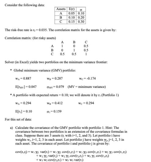
Consider the following data: Assets E(r) A B C 0 0.05 0.10 0.10 0.20 0.15 0.30 The risk-free rate is r = 0.035. The correlation matrix for the assets is given by: Correlation matrix: (for risky assets) A 1 B 0 1 0.5 0.5 1 A B C Solver (in Excel) yields two portfolios on the minimum variance frontier: * Global minimum variance (GMV) portfolio: Wa=0.287 0 0.5 0.5 WA=0.887 E[MV] -0.047 OMV 0.079 (MV-minimum variance) * A portfolio with expected return = 0.10; we will denote it by r. (Portfolio 1) WA = 0.294 Wa=0.412 Wc = 0.294 E[r] -0.10 0-0.159 For this set of data: We=-0.174 a) Calculate the covariance of the GMV portfolio with portfolio 1. Hint: The covariance between two portfolios is an extension of the covariance formulas in class. Suppose there are 3 assets (r, with i=1, 2, and 3). Let portfolio i have weights w, i 1, 2, 3 in each asset. Let portfolio j have weights w, j-1, 2, 3 in each asset. The covariance of portfolio i and portfolio j is given by: cov(n,r) w: Wi var(n)+wi w cov(n,r) + w ws cov(ri,rs)+W2 W cov(n,r) + W W var(r) + W W3 Cov(3) + W W (,) + W3 W2 Cov(rn) + WW var(r)