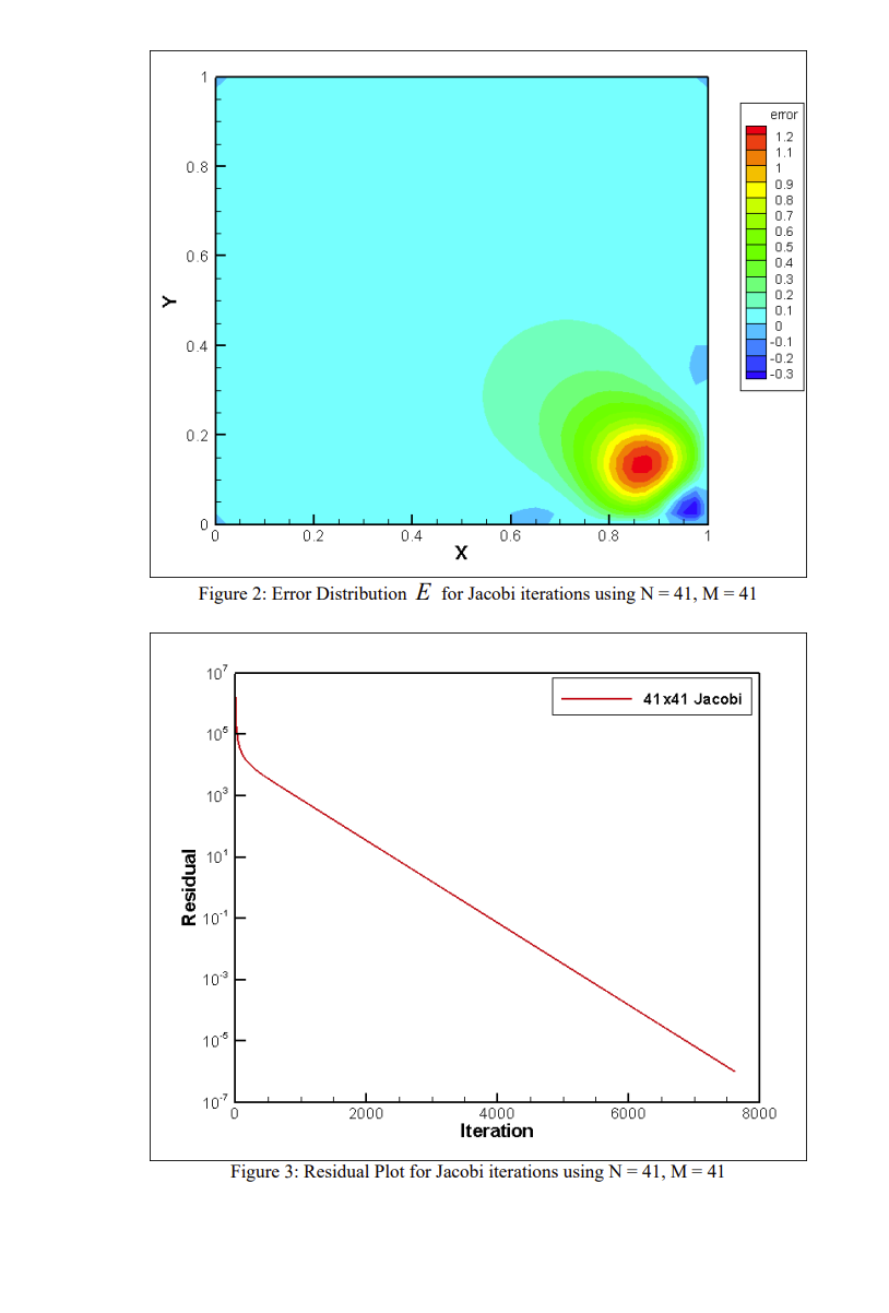
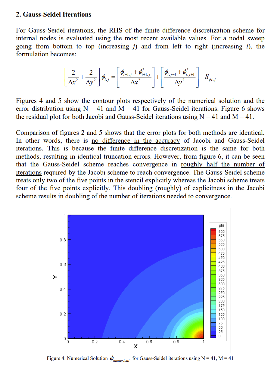
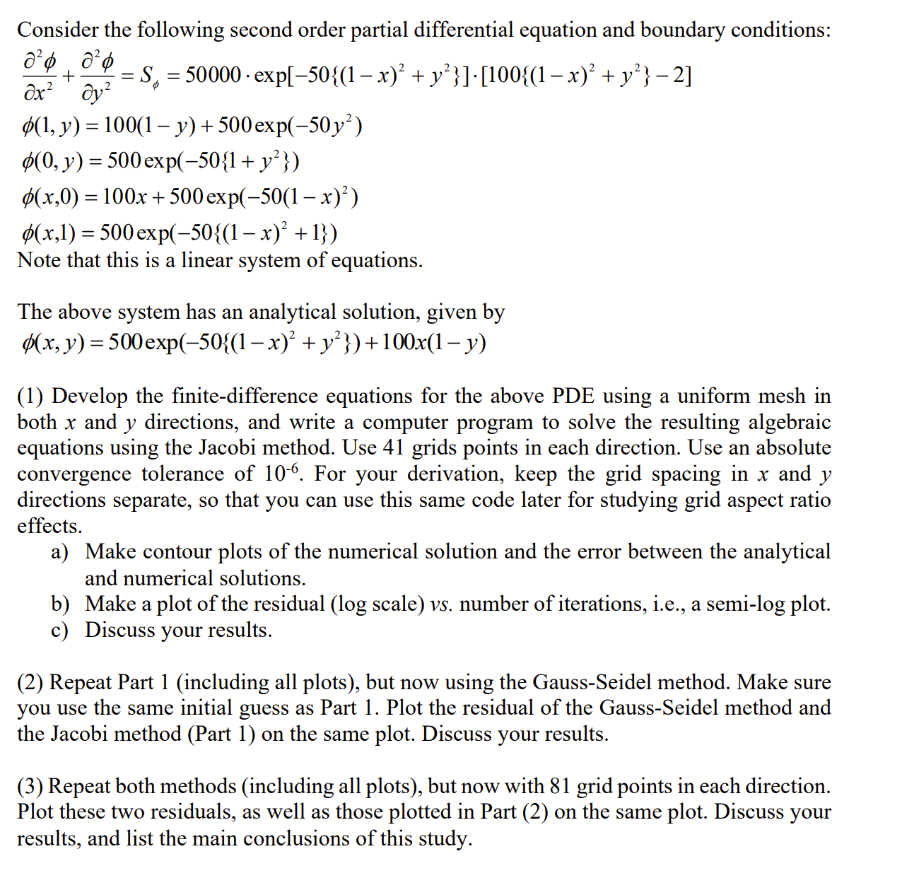
Consider the following second order partial differential equation and boundary conditions: 525:5 + 62:1: S, : 50000 -eXp[50{(1 x)2 +y2}]-[100{(1 x)2 + yz} 2] 6x 5y (1, y) 2100(17 y) + 500exp(750y2) (0,y) : 500 exp(750{l + y2}) (x,0) : 100x + 500 eXp(50(l x)2) (x,1): 500 eXp(50{(1 x)2 + 1}) Note that this is a linear system of equations. The above system has an analytical solution, given by 950:, y) = SOOeXp(50{(l x)2 + y2})+100x(1 y) (1) Develop the nite-difference equations for the above PDE using a uniform mesh in both x and y directions, and write a computer program to solve the resulting algebraic equations using the Jacobi method. Use 41 grids points in each direction. Use an absolute convergence tolerance of 10'\". For your derivation, keep the grid spacing in x and y directions separate, so that you can use this same code later for studying grid aspect ratio effects. a) Make contour plots of the numerical solution and the error between the analytical and numerical solutions. b) Make a plot of the residual (log scale) v5. number of iterations, Le, a semi-log plot. c) Discuss your results. (2) Repeat Part 1 (including all plots), but now using the Gauss-Seidel method. Make sure you use the same initial guess as Part 1. Plot the residual of the Gauss-Seidel method and the Jacobi method (Part 1) on the same plot. Discuss your results. (3) Repeat both methods (including all plots), but now with 81 grid points in each direction. Plot these two residuals, as well as those plotted in Part (2) on the same plot. Discuss your results, and list the main conclusions of this study. Governing Equation: = S =50000 . exp -50((1-x) +>}]. [100((1-x)+>}-2] Boundary Conditions: $(0, y) =500exp -50(1+ )?} ] $(1, y) =100(1-y)+500exp[-50y? ] $(x,0) =100x +500exp -50(1-x)] $ (x,1) =500 exp [- 50(1-x) + 1}] Analytical Solution: $(x, y) =500exp -50((1-x) + y?) +100x(1-y) Finite Difference Discretization The following discretization scheme assumes N nodes in the x-direction and M nodes in the y-direction. All through the following report, i and j represent indices in the x- and y- directions respectively. The coordinates of the nodes are given by: x; = (i-1)Ax = (i-1)-R_L= (i-1)- 1 N - 1 , i=1... N y; = (j-1)Ay = (j-1)- VB =(j-1) M-1 M- ' j= 1...M The boundary conditions are enforced using: For i = 1...N 9:1 =100x, +500 exp -50(1-x,)"] PM =500 exp -501(1-x,) + 1} ] For j = 1...M 4,; =500exp -50 (1+ y,?} ] $N./ =100(1-y,)+ 500 exp[-50y," ]Note that since Dirichlet boundary conditions for all boundaries are specified, it is not necessary to do iterations for the above nodes. We only need to solve for the internal nodes. The finite difference equations for the internal nodes are given by: For i = 2...(N-1) and j = 2...(M-1) 2 Ax2 The error between the analytical and numerical solutions is given by Eij = Panalytical i.j - 9numerical i,j 1. Jacobi Iterations For Jacobi iterations, the RHS of the finite difference discretization scheme for internal nodes is evaluated using values from the previous iteration (or initial guess for the first iteration). That is, the formulation for Jacobi iterations is given by: Figures 1 and 2 show the contour plots respectively of the numerical solution and the error distribution using N = 41 and M = 41 for Jacobi iterations. Figure 3 shows the residual plot for the same case. phi 600 575 0.8 550 525 500 475 450 425 0.6 400 375 350 325 300 04 275 250 225 200 175 150 J.2 125 100 75 50 25 0 0.2 0,4 0.6 0.8 X Figure 1: Numerical Solution numerical for Jacobi iterations using N = 41, M = 41emor 1.2 1.1 0.8 - 1 0.9 0.8 0.7 0.6 0.6 0.5 0.4 0.3 > 0.2 0.1 0.4 -0.1 0.2 -0.3 0.2 0.2 0.4 0.6 0.8 X Figure 2: Error Distribution E for Jacobi iterations using N = 41, M = 41 10 41x41 Jacobi 105 103 10' Residual D 101 103 105 10" 2000 4000 6000 8000 Iteration Figure 3: Residual Plot for Jacobi iterations using N = 41, M = 412. Gauss-Seidel Iterations For Gauss-Seidel iterations, the RHS of the finite difference discretization scheme for internal nodes is evaluated using the most recent available values. For a nodal sweep going from bottom to top (increasing j) and from left to right (increasing i), the formulation becomes: Ar Figures 4 and 5 show the contour plots respectively of the numerical solution and the error distribution using N = 41 and M = 41 for Gauss-Seidel iterations. Figure 6 shows the residual plot for both Jacobi and Gauss-Seidel iterations using N = 41 and M = 41. Comparison of figures 2 and 5 shows that the error plots for both methods are identical. In other words, there is no difference in the accuracy of Jacobi and Gauss-Seidel iterations. This is because the finite difference discretization is the same for both methods, resulting in identical truncation errors. However, from figure 6, it can be seen that the Gauss-Seidel scheme reaches convergence in roughly half the number of iterations required by the Jacobi scheme to reach convergence. The Gauss-Seidel scheme treats only two of the five points in the stencil explicitly whereas the Jacobi scheme treats four of the five points explicitly. This doubling (roughly) of explicitness in the Jacobi scheme results in doubling of the number of iterations needed to convergence. phi 600 575 0.8 550 525 500 475 450 425 0.6- 400 375 350 325 300 0.4 275 250 225 200 175 150 0.2 125 100 75 50 25 0.2 0,4 0.6 0.8 X Figure 4: Numerical Solution Pnumerical for Gauss-Seidel iterations using N = 41, M =41