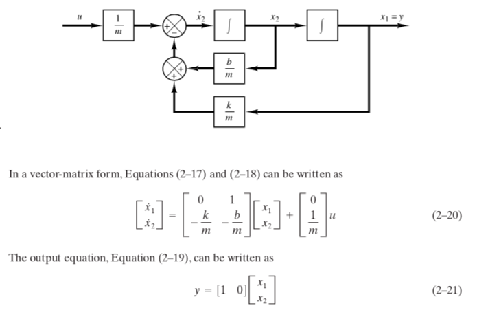
Consider the mechanical system in Example 2-2 on page 32 of the textbook, whose dynamics are described by (2-16)(2-21) and whose block diagram is shown in Figure 2-16. Suppose the system parameters are m = 1, b = 0.5, and k = 1, the system has no input (i.e., u(t) = 0 for all t 0), and the mass has an initial displacement of 2 and an initial velocity of 1 (i.e., x₁(0) = y(0) = 2 and x₂(0) = ydot(0) = 1). Calculate and plot the initial-condition response y(t) for t [0,25] in three equivalent ways:

(i) using ss and initial (do a help on initial);

(ii) using ss and lsim (with four input arguments); and

(iii) by creating a Simulink model that represents the block diagram in Figure 2-16. For (iii), to realize u(t) = 0 you may use the block Constant from the folder Sources and set Constant value to 0. To realize each integrator (integral) you may use the block Integrator from the folder Continuous and set Initial condition to 2 or 1. Check to make sure that your plots in (i)(iii) look identical.

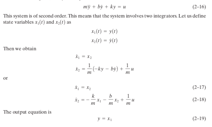
my + by + ky = u This system is of second order. This means that the system involves two integrators Let us define (2-16) state variables x1(t) and x2(t) as x(t)-y(t) Then we obtain -ky -bu or (2-17) (2-18) The output equation is (2-19) my + by + ky = u This system is of second order. This means that the system involves two integrators Let us define (2-16) state variables x1(t) and x2(t) as x(t)-y(t) Then we obtain -ky -bu or (2-17) (2-18) The output equation is (2-19)