Create an Excel workbook containing two depreciation schedule templates, each on a separate spreadsheet. One template should be a SL depreciation schedule and the other template should be a DDB depreciation schedule. You should construct the spreadsheets using the formulas and cell referencing so that when the value of input variables are altered the calculations which automatically adjust. The spreadsheet columns should include depreciation expense, accumulated depreciation, and book value end of year (see textbook 575-576 for examples). Please note, you can not depreciate assets below any salvage value, therefore you will need to use IF function (see IF function guidance below). You must construct the worksheet with the appropriate numeric format and professional layout. Round number values to the nearest whole dollar. The fixed variables for the assignment are as follows:

Life of asset = 10 years

Depreciation methods = straight-line or double-declining balance method

Purchase date of asset = January 1, 2018

I will test accuracy of your worksheet with random input variables acquisition cost and salvage value. Place your name in cell A1 of the worksheets. Review assignment rubric for specific grade evaluation.

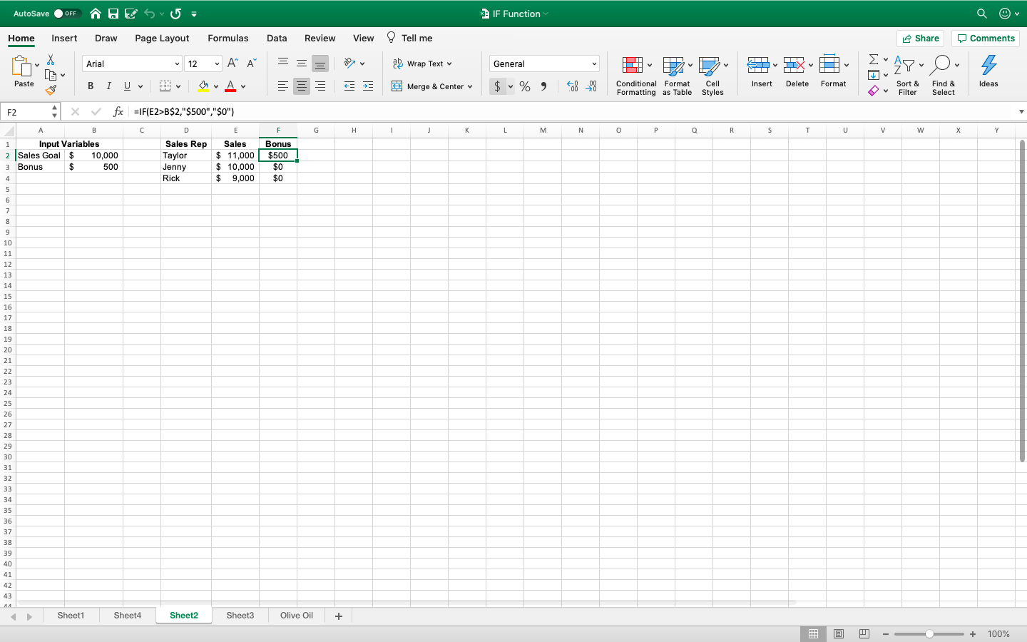
AutoSave OFF IF Function Home Insert Draw Page Layout Formulas Data Review View Tell me Share Comments X V v Arial 12 ~ AF ab Wrap Text General V Do SL LIX WE AYO s Paste B I U a. Av Merge & Center $ %) .00 .00 0 Insert Delete Format Conditional Format Formatting as Table Cell Styles Sort & Filter Ideas v Find & Select F2 fx =IF(E2>B$2,"$500","$0") E F G H 1 K L M N O P O R S T U V w X Y 1 A B Input Variables 2 Sales Goal $ 10,000 3 Bonus $ 500 4 5 6 7 8 9 D Sales Rep Taylor Jenny Rick Sales $ 11,000 $ 10,000 $ 9,000 Bonus $500 $0 $0 10 11 12 13 14 15 16 17 18 19 20 21 22 23 24 25 26 27 28 29 30 31 32 33 34 35 36 37 38 39 40 41 42 43 14 Sheet1 Sheet4 Sheet2 Sheet3 Olive Oil + 0 A + 100%