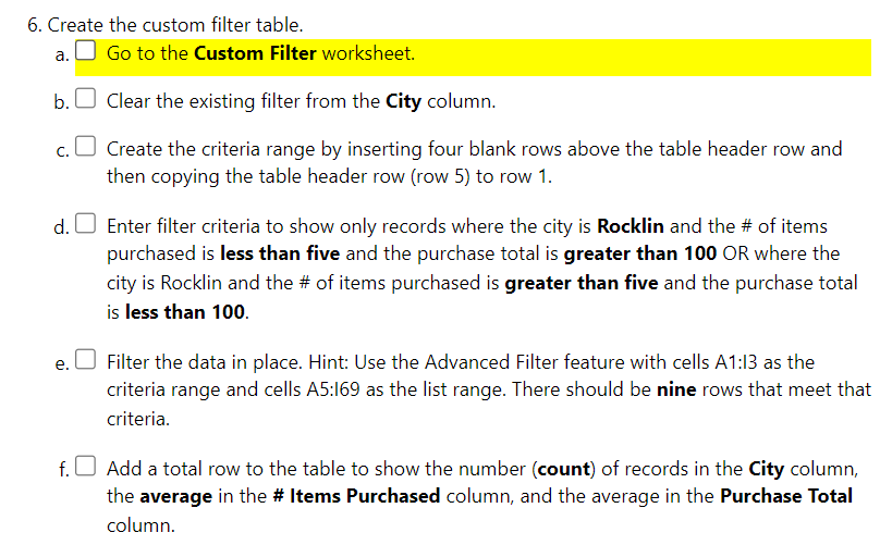
Create the custom filter table.

a$.$

Go to the Custom Filter worksheet.

b$.$ Clear the existing filter from the City column.

c$.$ Create the criteria range by inserting four blank rows above the table header row and

then copying the table header row $($row $5)$ to row $1.$

d$.$ Enter filter criteria to show only records where the city is Rocklin and the # of items

purchased is less than five and the purchase total is greater than $100$ OR where the

city is Rocklin and the # of items purchased is greater than five and the purchase total

is less than $100.$

e$.$ Filter the data in place. Hint: Use the Advanced Filter feature with cells A$1$:I$3$ as the

criteria range and cells A$5$:I$69$ as the list range. There should be nine rows that meet that

criteria.

f$.$ Add a total row to the table to show the number $($count$)$ of records in the City column,

the average in the # Items Purchased column, and the average in the Purchase Total

column.