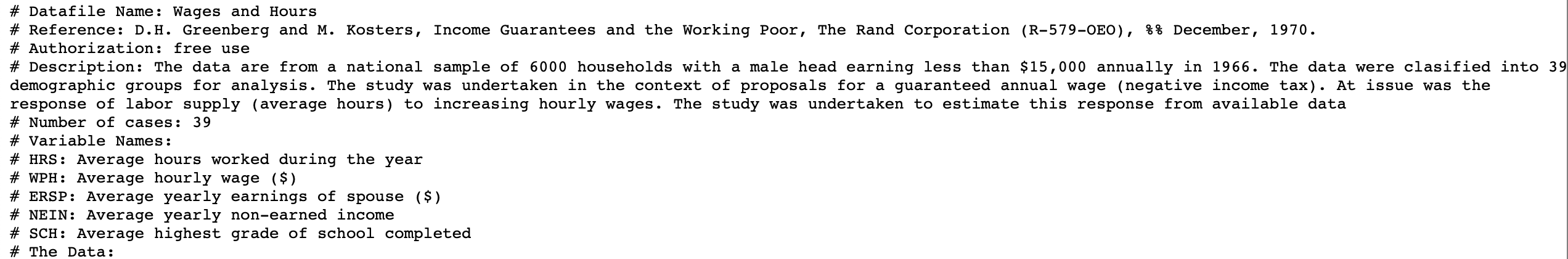
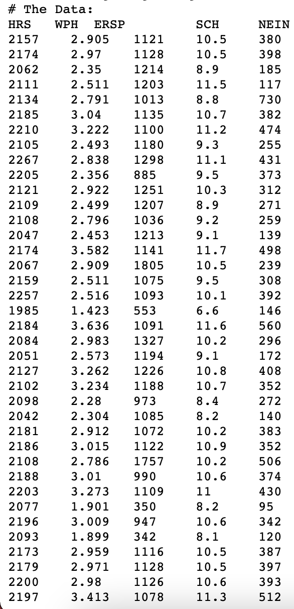
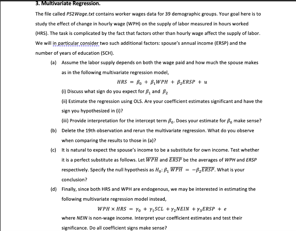
. # Datafile Name: Wages and Hours # Reference: D.H. Greenberg and M. Kosters, Income Guarantees and the Working Poor, The Rand Corporation (R-579-0EO), %% December, 1970. # Authorization: free use # Description: The data are from a national sample of 6000 households with a male head earning less than $15,000 annually in 1966. The data were clasified into 39 demographic groups for analysis. The study was undertaken in the context of proposals for a guaranteed annual wage (negative income tax). At issue was the response of labor supply (average hours) to increasing hourly wages. The study was undertaken to estimate this response from available data # Number of cases: 39 # Variable Names: # HRS: Average hours worked during the year # WPH: Average hourly wage ($) # ERSP: Average yearly earnings of spouse ($) # NEIN: Average yearly non-earned income # SCH: Average highest grade of school completed # The Data: # The Data: HRS WPH ERSP 2157 2.905 2174 2.97 2062 2.35 2111 2.511 2134 2.791 2185 3.04 2210 3.222 2105 2.493 2267 2.838 2205 2.356 2121 2.922 2109 2.499 2108 2.796 2047 2.453 2174 3.582 2067 2.909 2159 2.511 2257 2.516 1985 1.423 2184 3.636 2084 2.983 2051 2.573 2127 3.262 2102 3.234 2098 2.28 2042 2.304 2181 2.912 2186 3.015 2108 2.786 2188 3.01 2203 3.273 2077 1.901 2196 3.009 2093 1.899 2173 2.959 2179 2.971 2200 2.98 2197 3.413 1121 1128 1214 1203 1013 1135 1100 1180 1298 885 1251 1207 1036 1213 1141 1805 1075 1093 553 1091 1327 1194 1226 1188 973 1085 1072 1122 1757 990 1109 350 947 342 1116 1128 1126 1078 SCH 10.5 10.5 8.9 11.5 8.8 10.7 11.2 9.3 11.1 9.5 10.3 8.9 9.2 9.1 11.7 10.5 9.5 10.1 6.6 11.6 10.2 9.1 10.8 10.7 8.4 8.2 10.2 10.9 10.2 10.6 11 8.2 10.6 8.1 10.5 10.5 10.6 11.3 NEIN 380 398 185 117 730 382 474 255 431 373 312 271 259 139 498 239 308 392 146 560 296 172 408 352 272 140 383 352 506 374 430 95 342 120 387 397 393 512 3. Multivariate Regression. The file called PS2 Wage.txt contains worker wages data for 39 demographic groups. Your goal here is to study the effect of change in hourly wage (WPH) on the supply of labor measured in hours worked (HRS). The task is complicated by the fact that factors other than hourly wage affect the supply of labor. We will in particular consider two such additional factors: spouse's annual income (ERSP) and the number of years of education (SCH). (a) Assume the labor supply depends on both the wage paid and how much the spouse makes as in the following multivariate regression model, HRS = Bo + B.WPH + B2ERSP + u (i) Discuss what sign do you expect for B1 and B2 (ii) Estimate the regression using OLS. Are your coefficient estimates significant and have the sign you hypothesized in (i)? (iii) Provide interpretation for the intercept term Bo. Does your estimate for Bo make sense? (b) Delete the 19th observation and rerun the multivariate regression. What do you observe when comparing the results to those in (a)? (c) It is natural to expect the spouse's income to be a substitute for own income. Test whether it is a perfect substitute as follows. Let WPH and ERSP be the averages of WPH and ERSP respectively. Specify the null hypothesis as Ho:B, WPH = -B2ERSP. What is your conclusion? (d) Finally, since both HRS and WPH are endogenous, we may be interested in estimating the following multivariate regression model instead, WPH X HRS = Yo + Y1SCL + V2NEIN + Y3ERSP + e where NEIN is non-wage income. Interpret your coefficient estimates and test their significance. Do all coefficient signs make sense? . # Datafile Name: Wages and Hours # Reference: D.H. Greenberg and M. Kosters, Income Guarantees and the Working Poor, The Rand Corporation (R-579-0EO), %% December, 1970. # Authorization: free use # Description: The data are from a national sample of 6000 households with a male head earning less than $15,000 annually in 1966. The data were clasified into 39 demographic groups for analysis. The study was undertaken in the context of proposals for a guaranteed annual wage (negative income tax). At issue was the response of labor supply (average hours) to increasing hourly wages. The study was undertaken to estimate this response from available data # Number of cases: 39 # Variable Names: # HRS: Average hours worked during the year # WPH: Average hourly wage ($) # ERSP: Average yearly earnings of spouse ($) # NEIN: Average yearly non-earned income # SCH: Average highest grade of school completed # The Data: # The Data: HRS WPH ERSP 2157 2.905 2174 2.97 2062 2.35 2111 2.511 2134 2.791 2185 3.04 2210 3.222 2105 2.493 2267 2.838 2205 2.356 2121 2.922 2109 2.499 2108 2.796 2047 2.453 2174 3.582 2067 2.909 2159 2.511 2257 2.516 1985 1.423 2184 3.636 2084 2.983 2051 2.573 2127 3.262 2102 3.234 2098 2.28 2042 2.304 2181 2.912 2186 3.015 2108 2.786 2188 3.01 2203 3.273 2077 1.901 2196 3.009 2093 1.899 2173 2.959 2179 2.971 2200 2.98 2197 3.413 1121 1128 1214 1203 1013 1135 1100 1180 1298 885 1251 1207 1036 1213 1141 1805 1075 1093 553 1091 1327 1194 1226 1188 973 1085 1072 1122 1757 990 1109 350 947 342 1116 1128 1126 1078 SCH 10.5 10.5 8.9 11.5 8.8 10.7 11.2 9.3 11.1 9.5 10.3 8.9 9.2 9.1 11.7 10.5 9.5 10.1 6.6 11.6 10.2 9.1 10.8 10.7 8.4 8.2 10.2 10.9 10.2 10.6 11 8.2 10.6 8.1 10.5 10.5 10.6 11.3 NEIN 380 398 185 117 730 382 474 255 431 373 312 271 259 139 498 239 308 392 146 560 296 172 408 352 272 140 383 352 506 374 430 95 342 120 387 397 393 512 3. Multivariate Regression. The file called PS2 Wage.txt contains worker wages data for 39 demographic groups. Your goal here is to study the effect of change in hourly wage (WPH) on the supply of labor measured in hours worked (HRS). The task is complicated by the fact that factors other than hourly wage affect the supply of labor. We will in particular consider two such additional factors: spouse's annual income (ERSP) and the number of years of education (SCH). (a) Assume the labor supply depends on both the wage paid and how much the spouse makes as in the following multivariate regression model, HRS = Bo + B.WPH + B2ERSP + u (i) Discuss what sign do you expect for B1 and B2 (ii) Estimate the regression using OLS. Are your coefficient estimates significant and have the sign you hypothesized in (i)? (iii) Provide interpretation for the intercept term Bo. Does your estimate for Bo make sense? (b) Delete the 19th observation and rerun the multivariate regression. What do you observe when comparing the results to those in (a)? (c) It is natural to expect the spouse's income to be a substitute for own income. Test whether it is a perfect substitute as follows. Let WPH and ERSP be the averages of WPH and ERSP respectively. Specify the null hypothesis as Ho:B, WPH = -B2ERSP. What is your conclusion? (d) Finally, since both HRS and WPH are endogenous, we may be interested in estimating the following multivariate regression model instead, WPH X HRS = Yo + Y1SCL + V2NEIN + Y3ERSP + e where NEIN is non-wage income. Interpret your coefficient estimates and test their significance. Do all coefficient signs make sense