Dataset

The dataset is stored in a CSV file named 'diabetes $2.$ CSV$\text{'},$ which has been provided to you.

The dataset consists of observations on $442$ patients, with the mesponse of interest being a

quantitative measure of disesse progression one year after baseline. There are ten $(10)$

baseline input variables, age, sex, body mass index, average blood pressure, and sir blood

serum mescurments. The last variable $Y$ is the output.

Task:

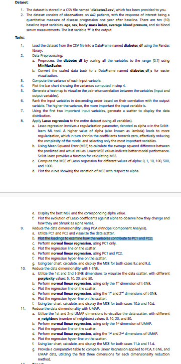
Lood the dataset fom the CSV file into a Dataframe named diabetes of using the Pandas

ibrary.

Data Preproceseing:

a$.$ Preproces the diabetes of by scaling all the variables to the range $0,1$ using

MinMaxscaler.

b$.$ Convert the scaled data back to a Dataframe named diabetes df s for easier

visualization.

Compute the variance of each input variable.

Plot the bar chart showing the varianoes computed in step $4.$

Generate a heatmap to visual ze the pair wise correlation between the variables $($input and

output variables$).$

Rank the input variables in descending order based on their correlation with the output

variable. The higher the variance, the more important the input variable is

Uaing the first two important input variables, generate a scatter to display the data

distribution.

Apply Lasso rogression to the entire dataset $($uaing all variables$).$

a$.$ Lasso regression involves a regularization parameter, dencted as alpha prop in the Scilat.

iesm ML tool. A higher value of aphs $($also known as lambda$)$ lesds to more

regulartaztion, which in tum shrinis the coefficients towards zero, effoctively reducing

the complenty of the model and selecting only the moet important variabies.

b$.$ Using Mean Squared ETror $($MSE$)$ to calculate the average squared difference between

the predicted and actual values. Lower MSE values indicate better model pertormanoe.

Scikit$-$leam provides a function for calaulating MSE.

c$.$ Compute the MSE of Laseo regression for different values of alphac: $0,1,10,100,500,$

and $1000.$

d$.$ Plat the curve showing the variation of MSE with respect to alpha.

e$.$ Display the best MSE and the corresponding alphe value

f$.$ Plat the evolution of Lasso coefficents against alpha to observe how they change and

how they are Shrunk as alpha varies.

Reduce the data dimensionality using PCA $($Principal Component Analysis$).$

a$.$ Utilise $PCl$ and $PC2$ and visualize the data scatter.

b$.$ Plot the losdings to examine how the variables contribute to PCI and PC$2.$

c$.$ Perform normal linear regression, uing PCI only.

d$.$ Plat the regression line on the scatter.

e$.$ Perform normal linear regression, using PCI and PC$2.$

t$.$ Plat the regression hyper$-$line on the scarter.

Using bar chart, calculate, and dsplay the M$5$E for both cases $9.$c and $9.$d$.$

Reduce the data dimensionality with $t-$ SNE.

a$.$ Utilise the $1$st and $2$nd t SNE dimensions to visualize the data scatter, with different

porplexity values $5,10,20,$ and $50.$

b$.$ Perform normal linear regression, using only the $1^n$ dimencion of $t$:SNE.

c$.$ Plot the regression line on the scatter.

d$.$ Pertomn normal linear regression, wing the $1^{al}$ and $2^{\text{n}\text{i}\text{t}}$ dimensions of $t5$ NE$.$

e$.$ Plat the regression hyper$-$line on the scarter.

t$.$ Using bar chart, calculate, and display the MSE for both cases $10.$b and $10.$d$.$

Reduce the data dimersionality with UMAP.

a$.$ Utiline the $1$st and $2$nd UMAP dimensions to visualize the data scatter, with different

n$\_$neighbors $($number of neighbors$)$ values $5,10,20,$ and $50.$

b$.$ Perform normal linear regression, ueing only the $1"$ dimencion of UMAP.

c$.$ Plat the regression line on the scatter.

d$.$ Portomn normal linear regression, uing the $1^{nl}$ and $2^{\text{n}\text{a}\text{l}}$ dimensions of UMAP.

e$.$ Plat the regression hyper$-$line on the scarter.

t$.$ Using bar chart, calculate, and display the MSE for both cases $11.$b and $11.$d$.$

Provide a comparative table to compare Linear Recression appled to RCA, t$-$SNE, and

UMAP data, usilizing the frst three dimensions for each dimeneionality reduction

method.