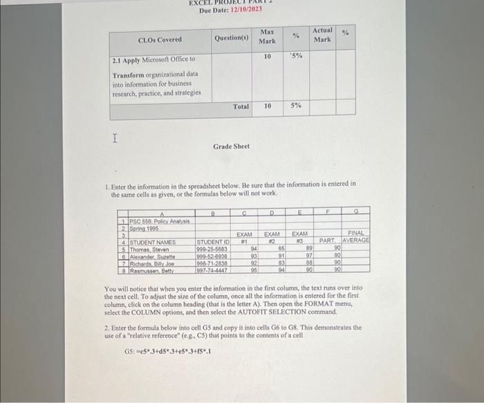
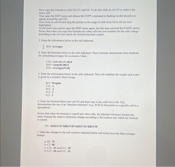
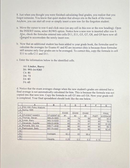
Dee Date: 12/10/2023 Grade Sheet 1. Enter the information in the spreadshect below. Be sure that the information is entered in the same cells as given, or the formulas below will not work. You will notice that when you enter the information in the first column, the text runs over into the next cell. To adjust the size of the column, once all the information is enterod for the first column, click on the column heading (that is the letter A). Then open the FORMAT menu, select the COLUMN options, and then select the AUTOFIT SELECTION command. 2. Enter the formula below into cell G5 and copy it into cells G6 to G8. This demonstrates the use of a "relative reference" (e.g., CS) that points to the eonients of a cell 65:=c3+d5.3+e5.3+15,1 Now copy this formula to cells G6, G7, and G8. To do this click on cell G5 to make it the active cell. Then open the EDIT menu and choose the COPY command (a flashing border should now appear around the cell G5). Now click on cell G6 and drag the pointer so the range of cells from G6 to G8 are now highlighted. At this point you need to open the EDTT menu again, but this time selected the PASTE option. Notice that when you copy this formula into other cells the row numbers for the cells change according to the row into which the formula has been copied. 3. Enter the information below in the cell indicated. I B10: Averages 4. Enter the formulas below in the cells indicated. These formulas demonstrate three methods for calculating averages for a column of data. C10:=(c5+c6+c7+c8)/4DI0:=sum(d5:d8)/4E10:-average(e5:e8) 5. Enter the information below in the cells indicated. This will establish the weight each exam is given in a student's final average. B12: Weights C12: 3 D12: 3 E12: 3 F12: 1 6. Enter the formula below into cell G5 and then copy it into cells G6 to G8. This demonstrates the use of an "absolute reference" (e.g, SCS12) that points to a specifie cell in a spreadsheet. Notice that when the formula is copied into other cells, the absolute reference remains the same whereas the relative references change according to the location into which the formula is copied. 7. Make the changes to the cell contents indicated below and notice how the final averages change. a. D5: 74 b. C7:98 c. C12:.25 and E12: .35 d. B12:30 and F12; 15 8. Just when you thought you were finished calculating final grades, you realize that you forgot someone, You know that quiet student that always sits in the back of the room. Anyhow, you can start all over or simply insert a new row for the forgotten student. a. Move the cursor to row 6 and click once (on any cell in this row or the row heading). Open the INSERT menu, select ROWS option. Notice how a new row is inserted after row 6 . Also, check the formulas entered into cells D11, E11, G5, G7, G8, and G9 have now all clilanged to accomodate the newly insert row. b. Now that an additional student has been added to your grade book, the formulas used to calculate the averages for Exams #1 and #2 are incorrect (this is because these formulas still assume only four grades are to be averaged. To correct this, copy the formula in cell E11 to cells C11 and D11. c. Enter the information below in the identified cells. A6:Linder,BarryB6:993149283C6:81D6:73E6:83F6:65 d. Notice that the exam averages change when the new student's grades are entered but a final average is not automatically calculated for him. This is because the formula was not copied into that new row. Copy the formula in cell G5 into cell G6. Now your grade roll is completed. Your final spreadsheet should look like the one below