1. Determine whether or not you will need a loan for each potential purchase.

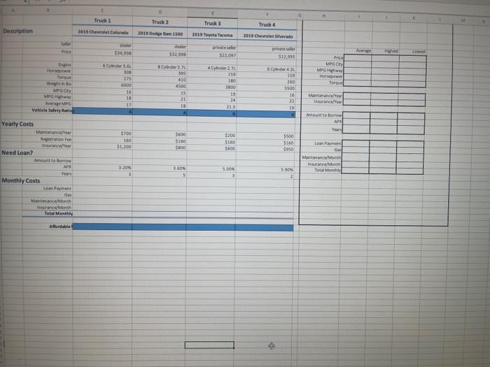
• Using absolute cell referencing as appropriate, in cell C21, enter a formula using an IF function to determine if you need a loan. Your available cash is located in cell A3 on the Data worksheet. If the price of the truck is less than or equal to your available cash, display, no, if not display yes.
• Copy the formula to the appropriate cells for the other trucks.

Calculate how much you would need to borrow for each purchase.

• In cell C22, enter a formula to calculate the price of the truck minus your available cash (from cell A3 in the Data worksheet). Use absolute references where appropriateyou will be copying this formula across the row.
• Copy the formula to the appropriate cells for the other trucks.

Calculate the monthly payment amount for each loan.

• In cell C26, enter a formula using the PMT function to calculate the monthly loan payment for the first truck. Hint: Divide the interest rate by 12 in the Rate argument to reflect monthly payments.
• Hint: Multiply the number of years by 12 in the Nper argument to reflect the number of monthly payments during the life of the loan. Hint: Use a negative value for the loan amount in the Pv argument so the payment amount is expressed as a positive number.
• Copy the formula to the appropriate cells for the other trucks.

Compute the monthly cost of gas.

• In cell C27, enter a formula to calculate the number of miles you expect to drive each month. Divide the value of number of miles (cell A5 from the Data sheet) by the average MPG for the vehicle multiplied by the price of a gallon of gas (cell A6 from the Data sheet).
• Copy the formula to the appropriate cells for the other trucks.
• If cells D27:F27 display an error or a value of 0, display formulas and check for errors.
• If you still cant find the error, try displaying the precedent arrows. Hint: The references to the cells on the Data sheet should use absolute references. If they do not, the formula will update incorrectly when you copy it across the row.

Compute the monthly cost of maintenance.

• In cell C28, enter a formula to calculate the monthly maintenance cost: Divide cell C18 by 12.
• Copy the formula to the appropriate cells for the other trucks.

Compute the monthly cost of insurance.

• In cell C29, enter a formula to calculate the monthly insurance cost: Divide cell C20 by 12.
• Copy the formula to the appropriate cells for the other trucks.

In cells C30:F30, compute the total the monthly cost for each truck.

Determine which trucks are affordable.

• Using absolute cell referencing as appropriate, in cell C32, enter a formula using an IF function to determine if the total monthly cost is less than or equal to the total monthly cost amount available for vehicle expenses. The total monthly cost is located in cell C30 on the Purchase worksheet. The total monthly cost amount available for vehicle expenses is located in cell A4 on the Data worksheet. If the total monthly cost is not less than or equal to the total monthly amount available, display no, if it is display yes.
• Copy the formula to the appropriate cells for the other trucks.
• Display formulas and use the error checking skills learned in this lesson to track down and fix any errors.

Complete the Analysis section using formulas with statistical functions. Use named ranges instead of cell references in the formulas.

• Price
• MPG City
• MPG Highway
• Horsepower
• Torque
• Maintenance/Year
• Insurance/Year
• Amount to Borrow
• APR
• Years
• Loan Payment
• Gas
• Maintenance/Month
• Insurance/Month
• Total Monthly

• Hint: Select cells B6:F30 and use Excels Create from Selection command to create named ranges for each row using the labels at the left side of the range as the names.
• Hint: Open the Name Manager and review the names Excel created. Notice that any spaces or special characters in the label names are converted to _ characters in the names.
• Hint: To avoid typos as you create each formula, try using Formula AutoComplete to select the correct range name.

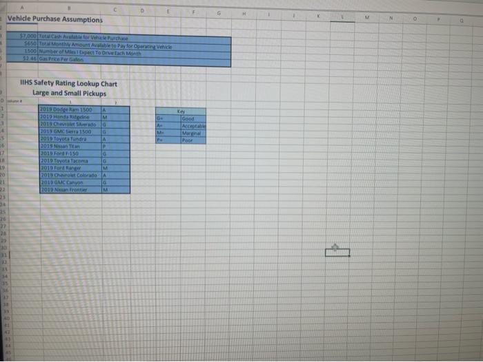
Vehicle Purchase Assumptions IIHS Safety Rating Lookup Chart Large and Small Pickups