1. determining the optimal advertising spend between options for the Chipotle account.

1. Articulate a hypothesis about which option(s) will have the greatest influence on sales performance.

1. Using the data set, run a multiple linear regression model in Excel.
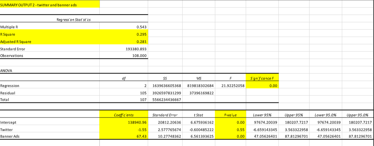
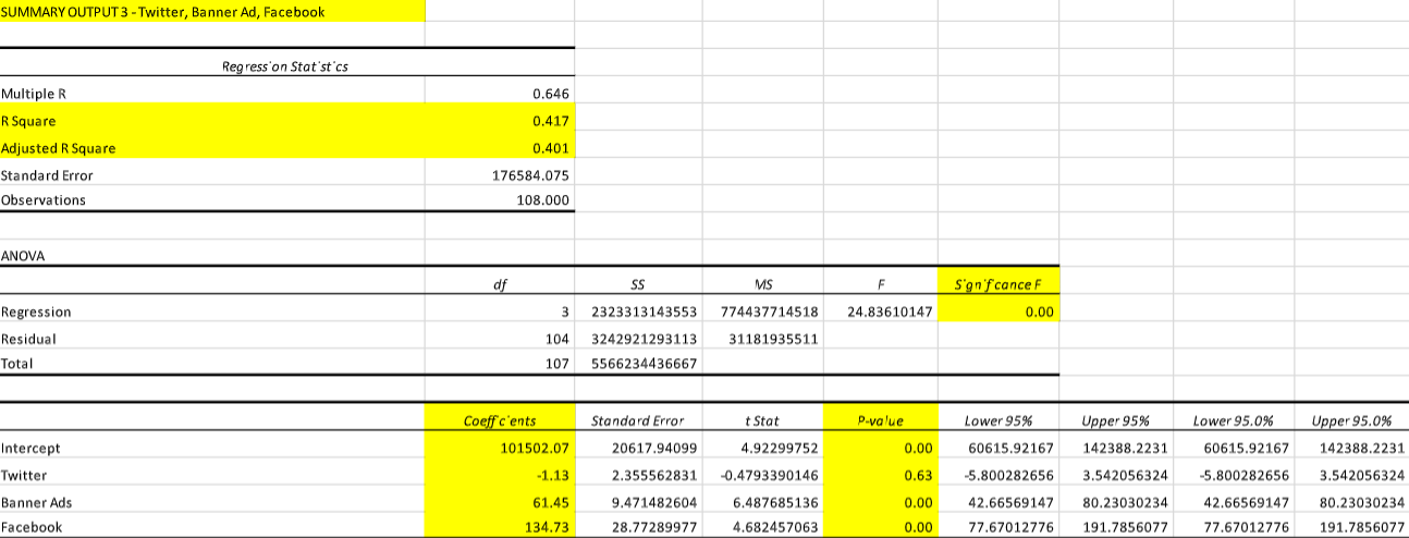
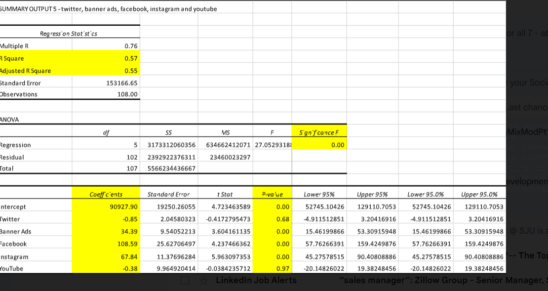
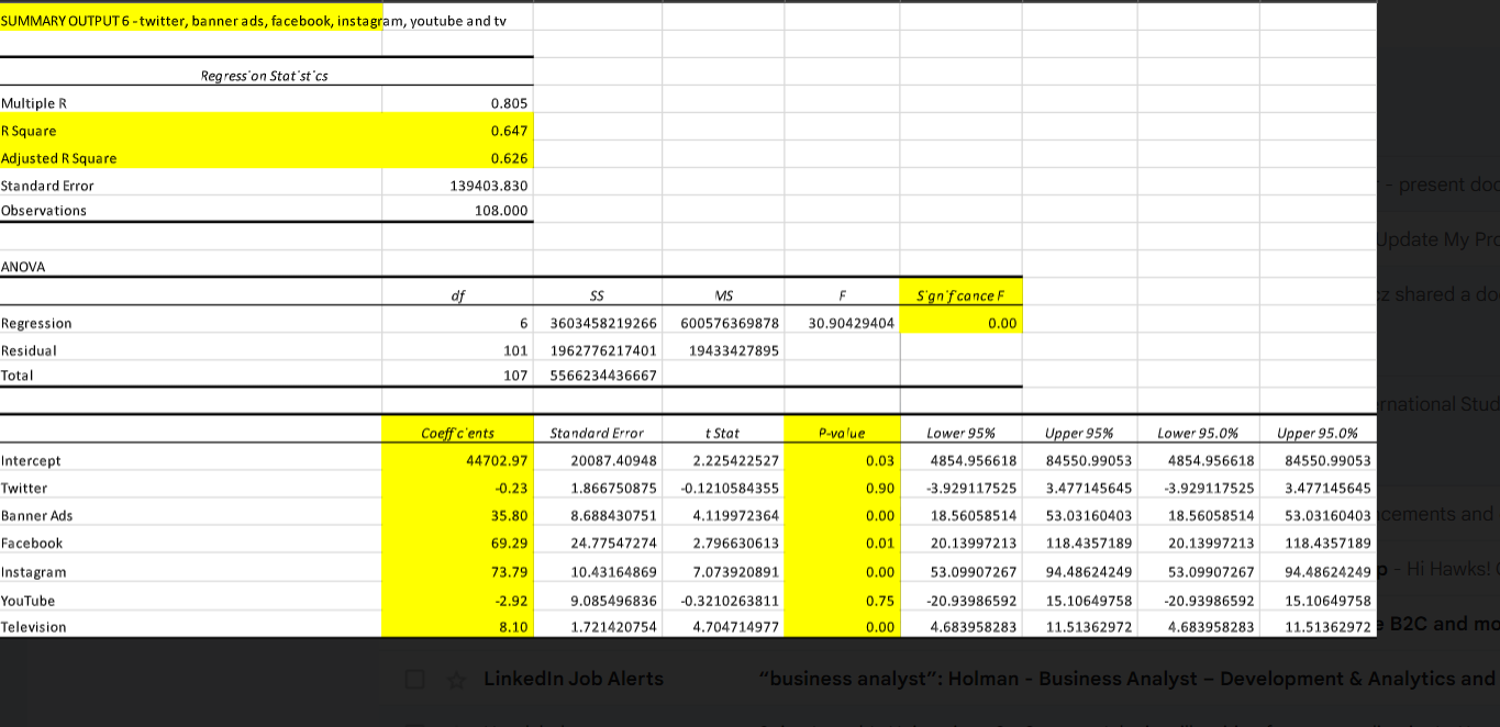
   1. Which advertising option(s) does your team recommend? [Hint: Which option (s) has a significant p-value? Which option(s) has the highest coefficient? ]
   2. How much increase in sales can your Chipotle client expect for a $10,000 increase in spending on your recommended option(s)?

please answer this immediately URGENT HELP NEEDED

SUMMARY OUTPUT 3 -Twitter, Banner Ad, Facebook \begin{tabular}{|c|c|c|c|c|c|c|c|} \hline 101502.07 & 20617.94099 & 4.92299752 & 0.00 & 60615.92167 & 142388.2231 & 60615.92167 & 142388.2231 \\ \hline \end{tabular} \begin{tabular}{|c|c|c|c|c|c|c|c|c|c|} \hline & Regress'on Stat 'st "cs & & & & & & & & \\ \hline Multiple R & & 0.805 & & & & & & & \\ \hline R Square & & 0.647 & & & & & & & \\ \hline Adjusted R Square & & 0.626 & & & & & & & \\ \hline Standard Error & & 139403.830 & & & & & & & \\ \hline Observations & & 108.000 & & & & & & & \\ \hline \multicolumn{10}{|l|}{ ANOVA } \\ \hline & & df & ss & MS & F & S'gn'fcance F & & & \\ \hline Regression & & 6 & 3603458219266 & 600576369878 & 30.90429404 & 0.00 & & & \\ \hline Residual & & 101 & 1962776217401 & 19433427895 & & & & & \\ \hline \multirow[t]{2}{*}{ Total } & & 107 & 5566234436667 & & & & & & \\ \hline & & Coeffcients & Standard Error & tStat & P-value & Lower 95\% & Upper 95\% & Lower 95.0\% & Upper 95.0\% \\ \hline Intercept & & 44702.97 & 20087.40948 & 2.225422527 & 0.03 & 4854.956618 & 84550.99053 & 4854.956618 & 84550.99053 \\ \hline Twitter & & -0.23 & 1.866750875 & -0.1210584355 & 0.90 & -3.929117525 & 3.477145645 & -3.929117525 & 3.477145645 \\ \hline Banner Ads & & 35.80 & 8.688430751 & 4.119972364 & 0.00 & 18.56058514 & 53.03160403 & 18.56058514 & 53.03160403 \\ \hline Facebook & & 69.29 & 24.77547274 & 2.796630613 & 0.01 & 20.13997213 & 118.4357189 & 20.13997213 & 118.4357189 \\ \hline Instagram & & 73.79 & 10.43164869 & 7.073920891 & 0.00 & 53.09907267 & 94.48624249 & 53.09907267 & 94.48624249 \\ \hline YouTube & & -2.92 & 9.085496836 & -0.3210263811 & 0.75 & -20.93986592 & 15.10649758 & -20.93986592 & 15.10649758 \\ \hline Television & & 8.10 & 1.721420754 & 4.704714977 & 0.00 & 4.683958283 & 11.51362972 & 4.683958283 & 11.51362972 \\ \hline \end{tabular} \begin{tabular}{|c|c|c|c|c|c|c|c|c|} \hline \multicolumn{9}{|c|}{ Regress'on Stat'st 'cs } \\ \hline Multiple R & 0.76 & & & & & & & \\ \hline Square & 0.57 & & & & & & & \\ \hline Adjusted R Square & 0.55 & & & & & & & \\ \hline Standard Error & 153166.65 & & & & & & & \\ \hline Observations & 108.00 & & & & & & & \\ \hline \multicolumn{9}{|l|}{ ANOVA } \\ \hline & df & sS & MS & F & S'gn'fcance F & & & \\ \hline Regression & 5 & 3173312060356 & 634662412071 & 27.05293181 & 0.00 & & & \\ \hline Residual & 102 & 2392922376311 & 23460023297 & & & & & \\ \hline Total & 107 & 5566234436667 & & & & & & \\ \hline & Coeffcents & Standard Error & tStat & P-value & Lower 95\% & Upper 95\% & Lower 95.0% & Upper 95.0\% \\ \hline ntercept & 90927.90 & 19250.26055 & 4.723463589 & 0.00 & 52745.10426 & 129110.7053 & 52745.10426 & 129110.7053 \\ \hline rwitter & -0.85 & 2.04580323 & -0.4172795473 & 0.68 & -4.911512851 & 3.20416916 & -4.911512851 & 3.20416916 \\ \hline Banner Ads & 34.39 & 9.54052213 & 3.604161135 & 0.00 & 15.46199866 & 53.30915948 & 15.46199866 & 53.30915948 \\ \hline acebook & 108.59 & 25.62706497 & 4.237466362 & 0.00 & 57.76266391 & 159.4249876 & 57.76266391 & 159.4249876 \\ \hline nstagram & 67.84 & 11.37696284 & 5.963097353 & 0.00 & 45.27578515 & 90.40808886 & 45.27578515 & 90.40808886 \\ \hline rouTube & -0.38 & 9.964920414 & -0.0384235712 & 0.97 & -20.14826022 & 19.38248456 & -20.14826022 & 19.38248456 \\ \hline \end{tabular} SUMMARY OUTPUT 4 - sales of twitter, banner ads, facebook and instagram \begin{tabular}{|c|c|c|c|c|c|c|c|c|} \hline & Regress'on Stat'st 'cs & & & & & & & \\ \hline Multiple R & 0.755 & & & & & & & \\ \hline R Square & 0.570 & & & & & & & \\ \hline Adjusted R Square & 0.553 & & & & & & & \\ \hline Standard Error & 152422.414 & & & & & & & \\ \hline Observations & 108.000 & & & & & & & \\ \hline \multicolumn{9}{|l|}{ ANOVA } \\ \hline & df & ss & MS & F & S'gnifcance F & & & \\ \hline Regression & 4 & 3173277424662 & 793319356165 & 34.14682891 & 0.00 & & & \\ \hline Residual & 103 & 2392957012005 & 23232592350 & & & & & \\ \hline \multirow[t]{2}{*}{ Total } & 107 & 5566234436667 & & & & & & \\ \hline & Coeffcients & Standard Error & t Stat & P-value & Lower 95\% & Upper 95\% & Lower 95.0% & Upper 95.0% \\ \hline Intercept & 90663.08 & 17886.81993 & 5.068708844 & 0.00 & 55188.79375 & 126137.371 & 55188.79375 & 126137.371 \\ \hline Twitter & -0.85 & 2.033778821 & -0.4179983361 & 0.68 & -4.883636778 & 3.183404451 & -4.883636778 & 3.183404451 \\ \hline Banner Ads & 34.32 & 9.325208673 & 3.679995859 & 0.00 & 15.8223773 & 52.81108131 & 15.8223773 & 52.81108131 \\ \hline Facebook & 108.74 & 25.20475453 & 4.314418692 & 0.00 & 58.75617814 & 158.73155 & 58.75617814 & 158.73155 \\ \hline Instagram & 67.90 & 11.22562037 & 6.048553155 & 0.00 & 45.63539112 & 90.16213189 & 45.63539112 & 90.16213189 \\ \hline \end{tabular} SUMMARY OUTPUT 3 -Twitter, Banner Ad, Facebook \begin{tabular}{|c|c|c|c|c|c|c|c|} \hline 101502.07 & 20617.94099 & 4.92299752 & 0.00 & 60615.92167 & 142388.2231 & 60615.92167 & 142388.2231 \\ \hline \end{tabular} \begin{tabular}{|c|c|c|c|c|c|c|c|c|c|} \hline & Regress'on Stat 'st "cs & & & & & & & & \\ \hline Multiple R & & 0.805 & & & & & & & \\ \hline R Square & & 0.647 & & & & & & & \\ \hline Adjusted R Square & & 0.626 & & & & & & & \\ \hline Standard Error & & 139403.830 & & & & & & & \\ \hline Observations & & 108.000 & & & & & & & \\ \hline \multicolumn{10}{|l|}{ ANOVA } \\ \hline & & df & ss & MS & F & S'gn'fcance F & & & \\ \hline Regression & & 6 & 3603458219266 & 600576369878 & 30.90429404 & 0.00 & & & \\ \hline Residual & & 101 & 1962776217401 & 19433427895 & & & & & \\ \hline \multirow[t]{2}{*}{ Total } & & 107 & 5566234436667 & & & & & & \\ \hline & & Coeffcients & Standard Error & tStat & P-value & Lower 95\% & Upper 95\% & Lower 95.0\% & Upper 95.0\% \\ \hline Intercept & & 44702.97 & 20087.40948 & 2.225422527 & 0.03 & 4854.956618 & 84550.99053 & 4854.956618 & 84550.99053 \\ \hline Twitter & & -0.23 & 1.866750875 & -0.1210584355 & 0.90 & -3.929117525 & 3.477145645 & -3.929117525 & 3.477145645 \\ \hline Banner Ads & & 35.80 & 8.688430751 & 4.119972364 & 0.00 & 18.56058514 & 53.03160403 & 18.56058514 & 53.03160403 \\ \hline Facebook & & 69.29 & 24.77547274 & 2.796630613 & 0.01 & 20.13997213 & 118.4357189 & 20.13997213 & 118.4357189 \\ \hline Instagram & & 73.79 & 10.43164869 & 7.073920891 & 0.00 & 53.09907267 & 94.48624249 & 53.09907267 & 94.48624249 \\ \hline YouTube & & -2.92 & 9.085496836 & -0.3210263811 & 0.75 & -20.93986592 & 15.10649758 & -20.93986592 & 15.10649758 \\ \hline Television & & 8.10 & 1.721420754 & 4.704714977 & 0.00 & 4.683958283 & 11.51362972 & 4.683958283 & 11.51362972 \\ \hline \end{tabular} \begin{tabular}{|c|c|c|c|c|c|c|c|c|} \hline \multicolumn{9}{|c|}{ Regress'on Stat'st 'cs } \\ \hline Multiple R & 0.76 & & & & & & & \\ \hline Square & 0.57 & & & & & & & \\ \hline Adjusted R Square & 0.55 & & & & & & & \\ \hline Standard Error & 153166.65 & & & & & & & \\ \hline Observations & 108.00 & & & & & & & \\ \hline \multicolumn{9}{|l|}{ ANOVA } \\ \hline & df & sS & MS & F & S'gn'fcance F & & & \\ \hline Regression & 5 & 3173312060356 & 634662412071 & 27.05293181 & 0.00 & & & \\ \hline Residual & 102 & 2392922376311 & 23460023297 & & & & & \\ \hline Total & 107 & 5566234436667 & & & & & & \\ \hline & Coeffcents & Standard Error & tStat & P-value & Lower 95\% & Upper 95\% & Lower 95.0% & Upper 95.0\% \\ \hline ntercept & 90927.90 & 19250.26055 & 4.723463589 & 0.00 & 52745.10426 & 129110.7053 & 52745.10426 & 129110.7053 \\ \hline rwitter & -0.85 & 2.04580323 & -0.4172795473 & 0.68 & -4.911512851 & 3.20416916 & -4.911512851 & 3.20416916 \\ \hline Banner Ads & 34.39 & 9.54052213 & 3.604161135 & 0.00 & 15.46199866 & 53.30915948 & 15.46199866 & 53.30915948 \\ \hline acebook & 108.59 & 25.62706497 & 4.237466362 & 0.00 & 57.76266391 & 159.4249876 & 57.76266391 & 159.4249876 \\ \hline nstagram & 67.84 & 11.37696284 & 5.963097353 & 0.00 & 45.27578515 & 90.40808886 & 45.27578515 & 90.40808886 \\ \hline rouTube & -0.38 & 9.964920414 & -0.0384235712 & 0.97 & -20.14826022 & 19.38248456 & -20.14826022 & 19.38248456 \\ \hline \end{tabular} SUMMARY OUTPUT 4 - sales of twitter, banner ads, facebook and instagram \begin{tabular}{|c|c|c|c|c|c|c|c|c|} \hline & Regress'on Stat'st 'cs & & & & & & & \\ \hline Multiple R & 0.755 & & & & & & & \\ \hline R Square & 0.570 & & & & & & & \\ \hline Adjusted R Square & 0.553 & & & & & & & \\ \hline Standard Error & 152422.414 & & & & & & & \\ \hline Observations & 108.000 & & & & & & & \\ \hline \multicolumn{9}{|l|}{ ANOVA } \\ \hline & df & ss & MS & F & S'gnifcance F & & & \\ \hline Regression & 4 & 3173277424662 & 793319356165 & 34.14682891 & 0.00 & & & \\ \hline Residual & 103 & 2392957012005 & 23232592350 & & & & & \\ \hline \multirow[t]{2}{*}{ Total } & 107 & 5566234436667 & & & & & & \\ \hline & Coeffcients & Standard Error & t Stat & P-value & Lower 95\% & Upper 95\% & Lower 95.0% & Upper 95.0% \\ \hline Intercept & 90663.08 & 17886.81993 & 5.068708844 & 0.00 & 55188.79375 & 126137.371 & 55188.79375 & 126137.371 \\ \hline Twitter & -0.85 & 2.033778821 & -0.4179983361 & 0.68 & -4.883636778 & 3.183404451 & -4.883636778 & 3.183404451 \\ \hline Banner Ads & 34.32 & 9.325208673 & 3.679995859 & 0.00 & 15.8223773 & 52.81108131 & 15.8223773 & 52.81108131 \\ \hline Facebook & 108.74 & 25.20475453 & 4.314418692 & 0.00 & 58.75617814 & 158.73155 & 58.75617814 & 158.73155 \\ \hline Instagram & 67.90 & 11.22562037 & 6.048553155 & 0.00 & 45.63539112 & 90.16213189 & 45.63539112 & 90.16213189 \\ \hline \end{tabular}