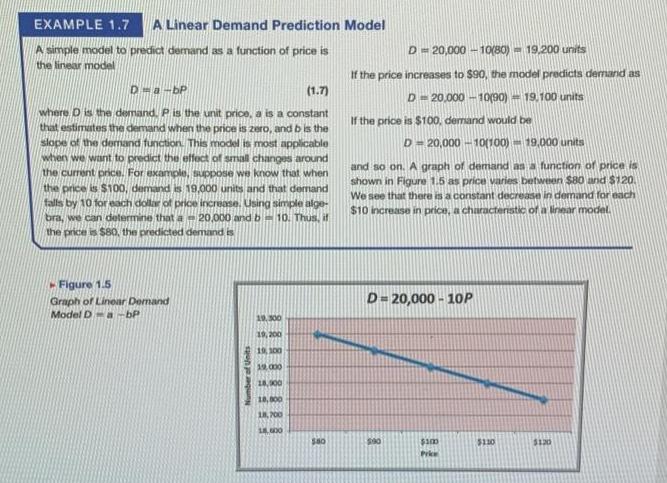
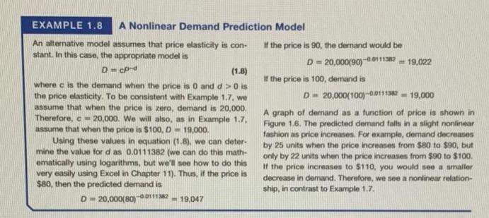
Develop a spreadsheet for computing the demand for any values of the input variables in the linear demand and nonlinear demand prediction models in Examples 1.7 and 1.8 in the chapter. EXAMPLE 1.7 A Linear Demand Prediction Model A simple model to predict demand as a function of price is the linear model D-a-bP (1.7) where D is the demand. P is the unit price, a is a constant that estimates the demand when the price is zero, and b is the slope of the demand function. This model is most applicable when we want to predict the effect of small changes around the current price. For example, suppose we know that when the price is $100, demand is 19,000 units and that demand falls by 10 for each dollar of price increase. Using simple alge- bra, we can determine that a 20,000 and b 10. Thus, if the price is $80, the predicted demand is Figure 1.5 Graph of Linear Demand Model D-a-bP Number of Units 19,300 19, 200 19, 100 19,000 18,900 10,000 18,700 18,000 $80 D=20,000-10(80) 19,200 units If the price increases to $90, the model predicts demand as D=20,000-10(90) 19,100 units If the price is $100, demand would be D=20,000-10(100) 19,000 units and so on. A graph of demand as a function of price is shown in Figure 1.5 as price varies between $80 and $120. We see that there is a constant decrease in demand for each $10 increase in price, a characteristic of a linear model. D=20,000-10P 5:90 $100 Price $110 $120 EXAMPLE 1.8 A Nonlinear Demand Prediction Model An alternative model assumes that price elasticity is con- stant. In this case, the appropriate model is D = ch (1.8) where c is the demand when the price is 0 and d> 0 is the price elasticity. To be consistent with Example 1.7, we assume that when the price is zero, demand is 20,000. Therefore, c20,000. We will also, as in Example 1.7, assume that when the price is $100, D- 19,000. Using these values in equation (1.8), we can deter- mine the value for d as 0.0111382 (we can do this math- ematically using logarithms, but we'll see how t do this very easily using Excel in Chapter 11). Thus, if the price is $80, then the predicted demand is D=20,000(80)-0.0111382 =19,047 If the price is 90, the demand would be D=20,000(90)-00111382 If the price is 100, demand is = 19,022 D 20,000(100)-0.011138219,000 A graph of demand as a function of price is shown in Figure 1.6. The predicted demand falls in a slight nonlinear fashion as price increases. For example, demand decreases by 25 units when the price increases from $80 to $90, but only by 22 units when the price increasies from $90 to $100. If the price increases to $110, you would see a smaller decrease in demand. Therefore, we see a nonlinear relation- ship, in contrast to Example 1.7.