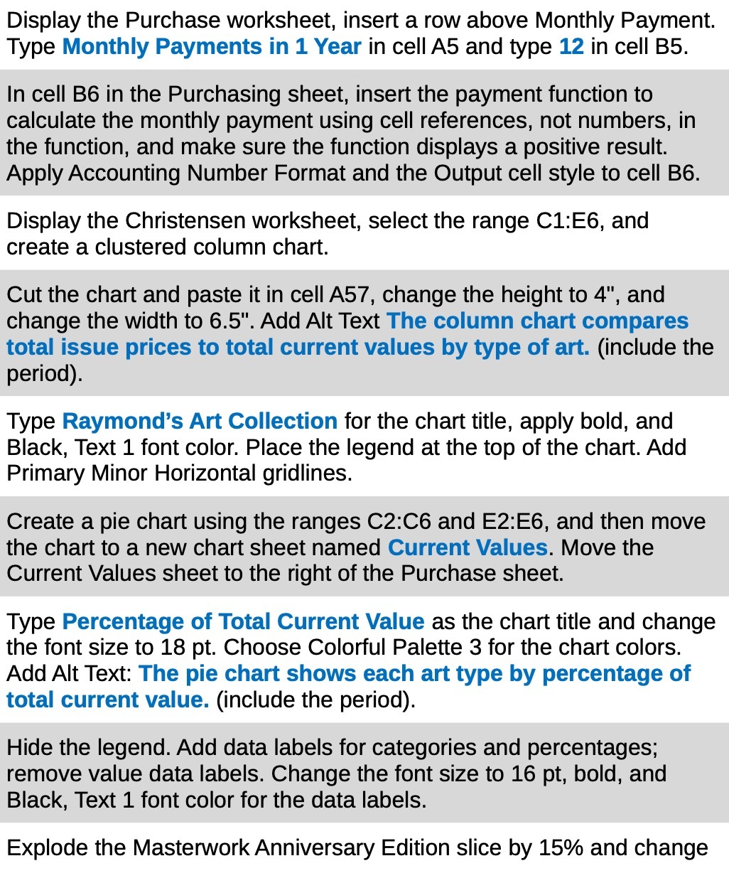
Display the Purchase worksheet, insert a row above Monthly Payment. Type Monthly Payments in 1 Year in cell A5 and type 12 in cell BS. In cell BS in the Purchasing sheet, insert the payment function to calculate the monthly payment using cell references, not numbers, in the function, and make sure the function displays a positive result. Apply Accounting Number Format and the Output cell style to cell BB. Display the Christensen worksheet, select the range C1:E6, and create a clustered column chart. Cut the chart and paste it in cell A57, change the height to 4", and change the width to 6.5". Add Alt Text The column chart compares total issue prices to total current values by type of art. (include the period). Type Raymond's Art Collection for the chart title, apply bold, and Black, Text 1 font color. Place the legend at the top of the chart. Add Primary Minor Horizontal gridlines. Create a pie chart using the ranges 02:06 and E2:E6, and then move the chart to a new chart sheet named Current Values. Move the Current Values sheet to the right of the Purchase sheet. Type Percentage of Total Current Value as the chart title and change the font size to 18 pt. Choose Colorful Palette 3 for the chart colors. Add Alt Text: The pie chart shows each art type by percentage of total current value. (include the period). Hide the legend. Add data labels for categories and percentages: remove value data labels. Change the font size to 16 pt, bold, and Black, Text 1 font color for the data labels. Explode the Masterwork Anniversary Edition slice by 15% and change