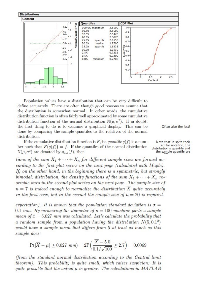
Distributions Content Quantiles CDF Plot 100.0% maximum 2.5500 .95- 99.5%% 2.5500 97.5% 2.5478 0.9- Normal Quantile Plot -1 .75 90.0% 2.3070 0.8- 75.0% quartile 2.0150 0.7 - 50-0 50.0% median 1.7700 .25- 25.0% quartile 1.6325 206- .10 10.0% 1.2530 2.5% 20.5- 0.7232 .05- 0.5. 0.7200 30.4- 0.0% minimum 0.7200 0.3- 0.2 - 15 2.5 Content Population values have a distribution that can be very difficult to define accurately. There are often though good reasons to assume that the distribution is somewhat normal. In other words, the cumulative distribution function is often fairly well approximated by some cumulative distribution function of the normal distribution N(#, o'). If in doubt, the first thing to do is to examine a graphical display. This can be Often also the last! done by comparing the sample quantiles to the relatives of the normal distribution. If the cumulative distribution function is F, its quantile q( f) is a num- Note that in spite their ber such that F(q(f)) = f. If the quantiles of the normal distribution similar notation, the distribution's quantile and N(p, o?) are denoted by qu.(f), then the sample quantile are tions of the sum X1+ ... + Xn for different sample sizes are formed ac- cording to the first plot series on the next page (calculated with Maple). If, on the other hand, in the beginning there is a symmetric, but strongly bimodal, distribution, the density functions of the sum X, + . . . + X, re- semble ones in the second plot series on the next page. The sample size of n = 7 is indeed enough to normalize the distribution X quite accurately in the first case, but in the second the sample size of n = 20 is required. expectation). It is known that the population standard deviation is o = 0.1 mm. By measuring the diameter of n = 100 machine parts a sample mean of I = 5.027 mm was calculated. Let's calculate the probability that a random sample from a population having the distribution N(5, 0.1?) would have a sample mean that differs from 5 at least as much as this sample does: P(|X - /| 2 0.027 mm) = 2P X - 5.0 0.1/ V100 2 2.7) = 0.0069 (from the standard normal distribution according to the Central limit theorem). This probability is quite small, which raises suspicion: It is quite probable that the actual u is greater. The calculations in MATLAB