Education quality is essential. You are given data on middle school students test performances in different districts in California in 1999. You would like to see how the reading and math test scores of students can be explained by some characteristics of the schools in the district. The response variable score is the average between reading and math scores. School characteristics (averaged across the district) include expenditures per student (expenditure), the percentage of students that qualify for a reduced price lunch (lunch), the percentage of students that are English learners (that is, students for whom English is a second language) (english), and district average income (in USD 1,000) (income). The data is as follows.

(a) You fit a model with the four predictors. Refer to the added variable plots presented in the printout. Interpret each of the added variable plots briefly.

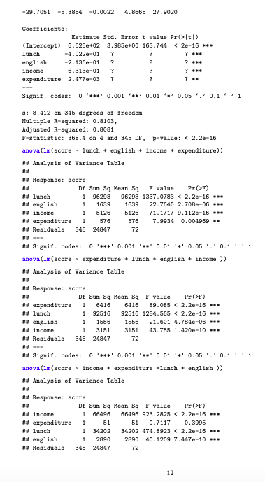
(b) Find the standard errors of the estimated coefficients for model1.

(c) Based on the negative slope coefficient for lunch, someone claims that the standard for receiving reduced price lunch should be raised, so that fewer students will qualify and thus the test scores will be higher. Comment on this claim.

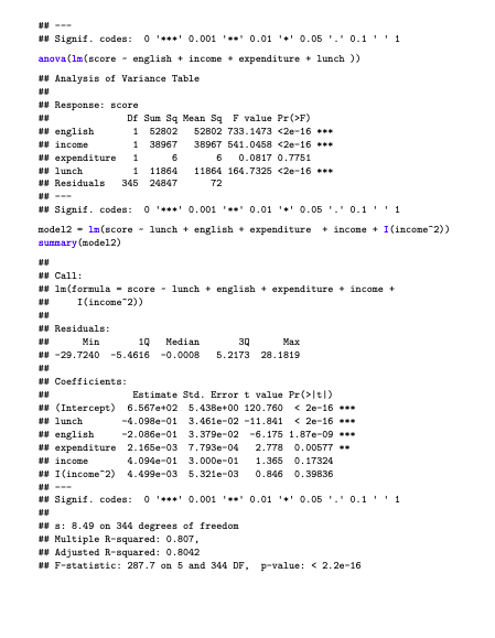
(d) You decide to add the squared term of income in model2. However, it seems that both first and second order terms are insignificant in the summary output. What could be the reason? Suggest a way that might solve this problem.

(e) Based on model2, what is the predicted average score for a new district whose characteristics are: lunch = 50, english = 50, income = 98, expenditure = 7800. Are there any concerns with this prediction?

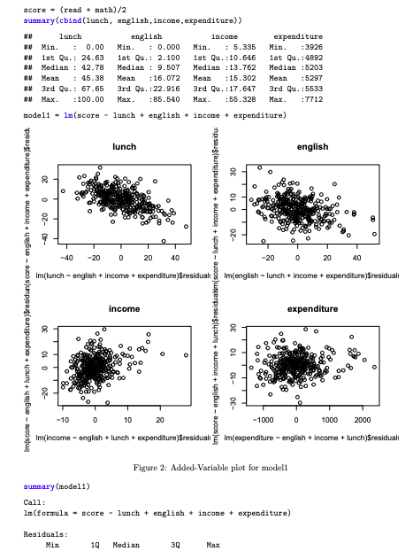
score - (read + math)/2 summary(cbind(lunch, english, income, expenditure) lunch english income expenditure Min. : 0.00 Min. : 0.000 Min. : 5.335 Min. : 3926 1st Qu.: 24.63 1st Qu.: 2.100 1st Qu.: 10.646 1st Qu.: 4892 Median : 42.78 Median : 9.507 Median :13.762 Median :5203 Mean : 45.38 Mean : 16.072 Mean : 15.302 Mean :5297 3rd Qu.: 67.65 3rd Qu.:22.916 3rd Qu. :17.647 3rd Qu.: 5533 . :100.00 Max. : 85.540 . :55.328 Max. :7712 modell - lm (score - lunch + english + income + expenditure) lunch english OE 010 o 08 9 -20 O -40 -20 0 20 40 -20 0 20 40 Im(lunch - english + income + expenditure)$residual Im(english - lunch + income + expenditure$residual 20 -40 -20 0 Imiscore - english + lunch + expenditure]Sresidun(score - english + income +expenditure residi 0 10 20 Im(score - english + income + lunch]$residualm(score - lunch + income + expenditure$residui income expenditure DE 30 -10 -30 -10 0 10 20 -1000 0 1000 2000 Im(income - english - lunch + expenditure)$residual Im(expenditure - english + income + lunch)$residual: Figure 2: Added Variable plot for modeli summary(modell) Call: 1m (formula - score - lunch + english + income + expenditure) Residuals: Min 10 Median 30 Max -29.7051 -5.3854 -0.0022 4.8665 27.9020 Coefficients: Estimate Std. Error t value Pr (>1tI) (Intercept) 6.525c+02 3.985e+00 163.744 F) W lunch 1 96298 96298 1337.0783 F) # expenditure 1 6416 6416 89.085 F) U income 1 66496 66496 923.2825 > W Analysis of Variance Table w Response: score DE Sum Sq Mean Sq F value Pr>F) w english 1 52802 52802 733. 1473 1tI) (Intercept) 6.525c+02 3.985e+00 163.744 F) W lunch 1 96298 96298 1337.0783 F) # expenditure 1 6416 6416 89.085 F) U income 1 66496 66496 923.2825 > W Analysis of Variance Table w Response: score DE Sum Sq Mean Sq F value Pr>F) w english 1 52802 52802 733. 1473