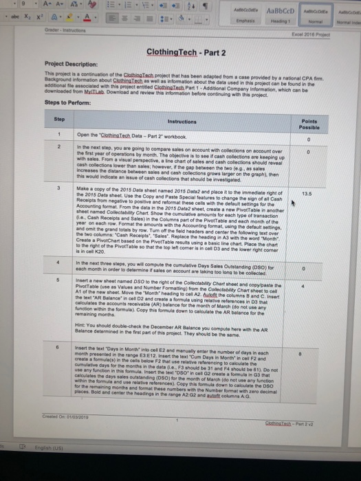
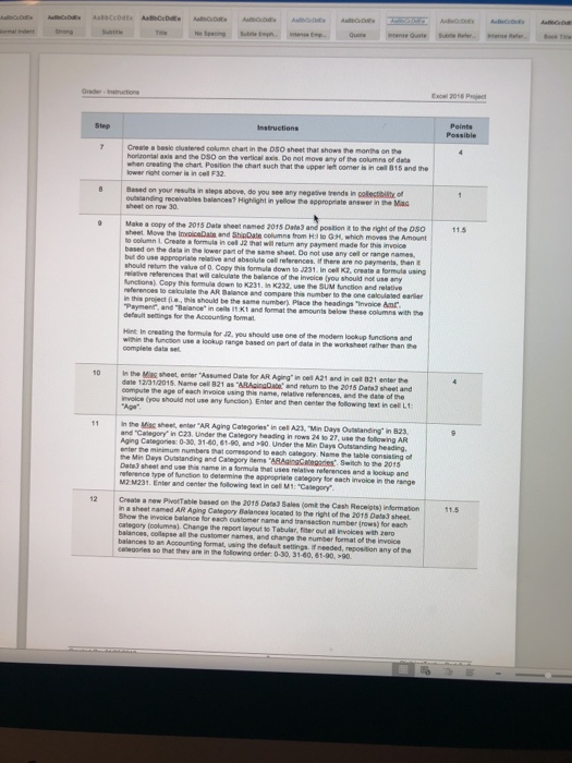
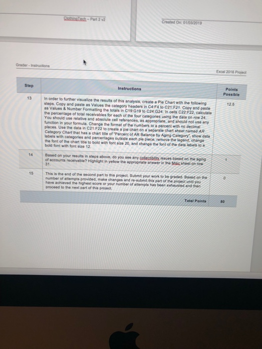
Enphasis Heading1 Excel 2016 Proj ClothingTech - Part 2 Project Description: This project is a continuation of the ClothinaTech project that has been adapted from a case provided by a national CPA fim Background information about ClthingTech additional le associated with this project entitied downloaded from MylTLab as well as information about the data used in this project can be found in the ClothingTach Part Additional Company Information, which can be Download and review this information before continuing with this project Steps to Perform: Points Possible Step Instructions 1 Open the ClothingTech Data- Part 2' workbook n the next step. you are going to compare sales on account with collections on account over with sales. From a visual year of operations by month. The objective is to see if cash collections are keeping up I perspective, a ine chart of sales and cash colections should reveal cash collections lower salers increases the distance between sales and cash than sales; however, if the gap between the two (e.g as sales collections grows larger on the graph then this would indicate an issue of cash collections that should be investigaed 3 Makecopy of the 2015 Date sheet named 201s Data2 and place t to the immedate righ of 13.5 the 2015 Date sheet Receipts from negative to positive and reformat these cells with the detauit settings for the Accounting format From the data in the sheet named Collectability Chart. Show the cumulative amounts for each type of (le., Cash Receipts and Sales) in the Columns part of the PivotTable and each month of the Use the Copy and Paste Special features to change the sign of all Cash 2015 Data2 sheet, create a new PivotTable in another f row. Format the amounts with the Accounting format, using the default seings and omit the grand totals by row. Tum of the feld headers and center the following text over Create a PivotChart based on the PivotTable results to the right of the PivotTable so that the top left comer is in cell D3 and the lower right corner using a basic line chart. Place the chart In the next three steps, you each month in order to determine if sales on account are will compute the cumulative Days Sales Outstanding (DSO) for taking too lona to be collected nsert a new sheet named DSO to the right of the Collectability Chart sheet and copyipaste the PivotTable (use as Values and Number Formatting) from the Collectabily Chart sheet to cell A1 of the new sheet. Move the text AR Balance* in cel D2 and create a formula using relative references in 03 that caloulates the accounts receivable (AR) balance for the month of March (do net use any function within the formula) Copy this formula down to calculabe the AR balance fer the remaining months. Hint You should double-check the December AR Balance you compute here with the AR Balance determined in the first part of this project. They should be the same nsert the text "Days in Month into cel E2 and manually enter the number of days in each month presented in the range E3 E12. Insert the text Cum Days in Month in cel F2 and a formula(s) in the cells below F2 that use relative referencing to calculate the oumulative days for the months in the data (Le, F3 should be 31 and F4 should be 61). Do o use any function in this formula. Insert the text 'DSO caloulates the days sales outstanding (DSO) for the month of March (do not use any within the formula and use relative references) for the remaining months and format these numbers with the Number format with zero places. Boid and center the headings in the range A2.32 and autofit columes A G In cel G2 ereate a formula in G3 that Copy this formula down to calculate the DSO decimal Created On: 01/03/2019 x 2016 Prject step basie clustered column chart in the DSO sheet that shows the months on the Create horizontal axis and the DSO on the vertical axis. Do not move any of the columns of when creating the chart Position the chart such that the upper let comer is in cell 815 and the Based on your nesults in steps above, do you see any negeive trends in collecticit of utstanding receivables balances? Highlight in yellow the appropiate answer in the Mi sheet on row 30 Make a copy of the 2015 Dats sheet named 2015 Date 3 and postion it to the right of the 0So sheet Move the InvoiceDatn and ShipDate columns from Hil lo G:, which moves the Amount ncel J2 fat w return any payment mado for this rvoe based on the but do use appropriate should returm the value of O Copy this formula down to J231. In cel kz, create a formule using n the lower part of the same sheet. Do not use any celtl or range names, hat will calculate the belance of the inweice (you should not use any unctions) Copy this formula down to K231. In K232. SUM function and nd compare this number to the one calculated earler n this project e tis Payment and "Baaner-in ces r, K, and format ne amounts bela. 9e" be the same number) Place the headings "invoice amr Hint In creating the formule for J2, you should use one of the moderm lookup functions and wihin the funcion use a lookup range based on part of data in the worksheet rather han 10 In the Ming sheet, enter "Assumed Date for AR Aging" in cel A21 and in cet 021 enter the date 1231/2015. Name cel 821 as "&BAsingDate and retum to the 2015 Date3 sheet and invoice (you should not use any funcsion) Enter and then center the folowing bext in cel L1 11 In the Miac shee, enter "AR Aging Categories"in cell A23, "Min Days Outstanding in 823, 0-30, 31-80, 61-90, and >90. Under the Min Days Outstanding headieg. references and a lookup and and "Category in C23. Under the Category heading in rows 24 to 27, use the following AR Aging Categories: the Min Days Ouistanding and Category items BAgiogGategades Sitch to the 2015 MZ M231. Enter and center the following text in cel M1: "Casegory n a sheet mamed AR Aging Category Balances located to the right of the 2015 Dats3 sheet sheet and use this name in a formula that uses relative of function to determine the appropriate canegory for each invoice in the range a new PivetTable besed on the 2015 Date3 Sales (omit the Cash Receipts) information Show the invoice balance category (ookumna). Change the report layout to Tabulb ustomer name and transaction number (rows) for er balances, colapse all the balances to an Accounting format, uaing the detault settings. if needed, reposition any of the ceteaornies so that they are in the following order 0-30, 31-60. 61-90, 90 names, and change the number foermat of the invoice Created On: 01/03/2019 Grader- Instructions Excel 2016 Project Points Possible Step Instructions 13 In order to further visualize the results of this analysis, create a Pie Chart with the following 12.5 steps. Copy and paste as values the category headers in C4 F4 to C21:F21 Copy and paste as values & Number Formatting the totals in C19:G19 to C24:G24 In ce is C22:F22. calculate ! the percentage of total receivables for each of the four categories using the data on row 24 You should use relative and absolute cell references, as appropriate, and should not use any function in your formula. Change the format of the numbers to a percent with no decimal places. Use the data in C21:F22 to create a ple chart on a separate chart sheet named AR Category Chart that has a chart title of "Percent of AR Balance by Aging Category, show data labels with categories and percentages outside each pie piece, remove the legend, change the font of the chant title to bold with font size 20, and change the font of the data labels to a bold font with font size 12. Based on your results in steps above, do you see any cetestibality, issues based on the aging of accounts receivable? Highlight in yellow the appropriate answer in the Misc sheet on row 31 This is the end of the second part to this project Submit your work to be graded. Based on the number of attempts provided, make changes and re-submit this part of the project untl you 15 have achieved the highest score or your number of attempts has been exhaussed and thon proceed to the next part of this project Total Points 80 Enphasis Heading1 Excel 2016 Proj ClothingTech - Part 2 Project Description: This project is a continuation of the ClothinaTech project that has been adapted from a case provided by a national CPA fim Background information about ClthingTech additional le associated with this project entitied downloaded from MylTLab as well as information about the data used in this project can be found in the ClothingTach Part Additional Company Information, which can be Download and review this information before continuing with this project Steps to Perform: Points Possible Step Instructions 1 Open the ClothingTech Data- Part 2' workbook n the next step. you are going to compare sales on account with collections on account over with sales. From a visual year of operations by month. The objective is to see if cash collections are keeping up I perspective, a ine chart of sales and cash colections should reveal cash collections lower salers increases the distance between sales and cash than sales; however, if the gap between the two (e.g as sales collections grows larger on the graph then this would indicate an issue of cash collections that should be investigaed 3 Makecopy of the 2015 Date sheet named 201s Data2 and place t to the immedate righ of 13.5 the 2015 Date sheet Receipts from negative to positive and reformat these cells with the detauit settings for the Accounting format From the data in the sheet named Collectability Chart. Show the cumulative amounts for each type of (le., Cash Receipts and Sales) in the Columns part of the PivotTable and each month of the Use the Copy and Paste Special features to change the sign of all Cash 2015 Data2 sheet, create a new PivotTable in another f row. Format the amounts with the Accounting format, using the default seings and omit the grand totals by row. Tum of the feld headers and center the following text over Create a PivotChart based on the PivotTable results to the right of the PivotTable so that the top left comer is in cell D3 and the lower right corner using a basic line chart. Place the chart In the next three steps, you each month in order to determine if sales on account are will compute the cumulative Days Sales Outstanding (DSO) for taking too lona to be collected nsert a new sheet named DSO to the right of the Collectability Chart sheet and copyipaste the PivotTable (use as Values and Number Formatting) from the Collectabily Chart sheet to cell A1 of the new sheet. Move the text AR Balance* in cel D2 and create a formula using relative references in 03 that caloulates the accounts receivable (AR) balance for the month of March (do net use any function within the formula) Copy this formula down to calculabe the AR balance fer the remaining months. Hint You should double-check the December AR Balance you compute here with the AR Balance determined in the first part of this project. They should be the same nsert the text "Days in Month into cel E2 and manually enter the number of days in each month presented in the range E3 E12. Insert the text Cum Days in Month in cel F2 and a formula(s) in the cells below F2 that use relative referencing to calculate the oumulative days for the months in the data (Le, F3 should be 31 and F4 should be 61). Do o use any function in this formula. Insert the text 'DSO caloulates the days sales outstanding (DSO) for the month of March (do not use any within the formula and use relative references) for the remaining months and format these numbers with the Number format with zero places. Boid and center the headings in the range A2.32 and autofit columes A G In cel G2 ereate a formula in G3 that Copy this formula down to calculate the DSO decimal Created On: 01/03/2019 x 2016 Prject step basie clustered column chart in the DSO sheet that shows the months on the Create horizontal axis and the DSO on the vertical axis. Do not move any of the columns of when creating the chart Position the chart such that the upper let comer is in cell 815 and the Based on your nesults in steps above, do you see any negeive trends in collecticit of utstanding receivables balances? Highlight in yellow the appropiate answer in the Mi sheet on row 30 Make a copy of the 2015 Dats sheet named 2015 Date 3 and postion it to the right of the 0So sheet Move the InvoiceDatn and ShipDate columns from Hil lo G:, which moves the Amount ncel J2 fat w return any payment mado for this rvoe based on the but do use appropriate should returm the value of O Copy this formula down to J231. In cel kz, create a formule using n the lower part of the same sheet. Do not use any celtl or range names, hat will calculate the belance of the inweice (you should not use any unctions) Copy this formula down to K231. In K232. SUM function and nd compare this number to the one calculated earler n this project e tis Payment and "Baaner-in ces r, K, and format ne amounts bela. 9e" be the same number) Place the headings "invoice amr Hint In creating the formule for J2, you should use one of the moderm lookup functions and wihin the funcion use a lookup range based on part of data in the worksheet rather han 10 In the Ming sheet, enter "Assumed Date for AR Aging" in cel A21 and in cet 021 enter the date 1231/2015. Name cel 821 as "&BAsingDate and retum to the 2015 Date3 sheet and invoice (you should not use any funcsion) Enter and then center the folowing bext in cel L1 11 In the Miac shee, enter "AR Aging Categories"in cell A23, "Min Days Outstanding in 823, 0-30, 31-80, 61-90, and >90. Under the Min Days Outstanding headieg. references and a lookup and and "Category in C23. Under the Category heading in rows 24 to 27, use the following AR Aging Categories: the Min Days Ouistanding and Category items BAgiogGategades Sitch to the 2015 MZ M231. Enter and center the following text in cel M1: "Casegory n a sheet mamed AR Aging Category Balances located to the right of the 2015 Dats3 sheet sheet and use this name in a formula that uses relative of function to determine the appropriate canegory for each invoice in the range a new PivetTable besed on the 2015 Date3 Sales (omit the Cash Receipts) information Show the invoice balance category (ookumna). Change the report layout to Tabulb ustomer name and transaction number (rows) for er balances, colapse all the balances to an Accounting format, uaing the detault settings. if needed, reposition any of the ceteaornies so that they are in the following order 0-30, 31-60. 61-90, 90 names, and change the number foermat of the invoice Created On: 01/03/2019 Grader- Instructions Excel 2016 Project Points Possible Step Instructions 13 In order to further visualize the results of this analysis, create a Pie Chart with the following 12.5 steps. Copy and paste as values the category headers in C4 F4 to C21:F21 Copy and paste as values & Number Formatting the totals in C19:G19 to C24:G24 In ce is C22:F22. calculate ! the percentage of total receivables for each of the four categories using the data on row 24 You should use relative and absolute cell references, as appropriate, and should not use any function in your formula. Change the format of the numbers to a percent with no decimal places. Use the data in C21:F22 to create a ple chart on a separate chart sheet named AR Category Chart that has a chart title of "Percent of AR Balance by Aging Category, show data labels with categories and percentages outside each pie piece, remove the legend, change the font of the chant title to bold with font size 20, and change the font of the data labels to a bold font with font size 12. Based on your results in steps above, do you see any cetestibality, issues based on the aging of accounts receivable? Highlight in yellow the appropriate answer in the Misc sheet on row 31 This is the end of the second part to this project Submit your work to be graded. Based on the number of attempts provided, make changes and re-submit this part of the project untl you 15 have achieved the highest score or your number of attempts has been exhaussed and thon proceed to the next part of this project Total Points 80