EXC$19$E$1-$ Practical Component Instructions

Complete the practical component by following these instructions. You will use your completed practical

component to answer $10$ questions on the online test, but you will not submit or upload the practical

component in myAOLCC.

Please return these instructions and your completed practical component to your Learning Coach once

you have completed the online test.

Please note that these are general and not step$-$by$-$step instructions. In this practical component, you

will use Microsoft Excel $2019$ to perform the following functions:

$$ formatting

$$ adding and replacing information in the worksheet

$$ creating formulas

$$ adding footers

$$ copying data to another worksheet

Instructions

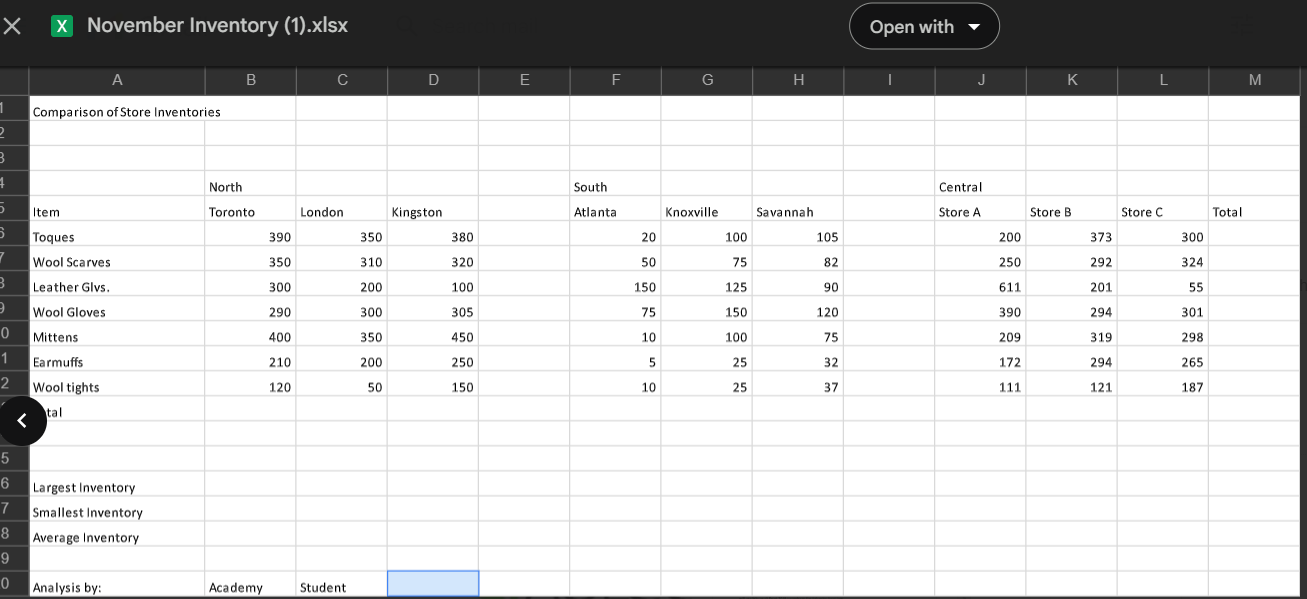
$1.$ Open the workbook, November Inventory.xlsx$,$ which will be provided to you by your Learning

Coach.

$2.$ Add the text, $$ Week Ending November $16,$ to the title in cell A$1.$

$3.$ Now apply the Heading $1$ style to the title, Comparison of Store Inventories $$ Week Ending

November $16.$

$4.$ In cell A$2,$ add the subtitle, Cold Weather Wear. Apply the Heading $2$ style.

$5.$ Change the label in cell A$7$ from Wool Scarves to Scarves.

$6.$ Change the label in cell B$4$ from North to East.

$7.$ For the Central area, change the labels Store A$,$ Store B$,$ and Store C to the labels New York,

Pittsburgh, and Buffalo respectively.

$8.$ Change the width for columns E and I to $3\mathrm{.}00.$

$9.$ Insert a row below the Toques row. Add the label Dress Hats in the first cell in this new row.

$10.$ On the Dress Hats row, add the data as shown:

Item Toronto London Kingston Atlanta Knoxville Savannah New York Pittsburgh Buffalo

Dress Hats $203119724908088333108119$

$11.$ Bold all the labels in rows $4,5,14,17,18,$ and $19.($Note: Bold only the labels, e$.$g$.,$ East, South,

Central; not all the cells in those rows.$)$

$2$

$12.$ Italicize the names of the products in column A $($Hats$,$ Scarves, etc.$).$

$13.$ Merge and center cells B$4,$ C$4,$ and D$4.$ Do the same for cells F$4,$ G$4,$ H$4,$ and for cells J$4,$ K$4,$ and L$4.$

$14.$ In row $14,$ use the SUM function to create a formula that totals the figures in columns B$,$ C$,$ D$,$ F$,$ G$,$

H$,$ J$,$ K$,$ and L$.$ For example, create a formula in cell B$14$ that totals cells B$6$:B$13,$ etc.

$15.$ In column M$,$ use AutoSum to total the figures in rows $6$ to $13.$ For example, in cell M$6$ use

AutoSum to total cells B$6$:L$6,$ etc.

$16.$ In cell M$14,$ create a formula without using a function to add up the values in cell B$14,$ C$14,$ D$14,$

F$14,$ G$14,$ H$14,$ J$14,$ K$14,$ and L$14.$

$17.$ In row $14,$ add a border to the totals with a single line on top and a double line below.

$18.$ Format all the numbers with a comma and no decimal places.

$19.$ AutoFit columns B to M$.$

$20.$ Fill the range M$6$:M$14$ with the Dark Blue, Text $2,$ Lighter $80\%$ color.

$21.$ Use functions to create formulas in cells C$17,$ C$18,$ and C$19$ respectively to calculate the Highest,

Lowest, and Average Inventory. These numbers should also have no decimal places.

$22.$ Use the CONCAT function in cell A$3$ to join cell B$21$ and cell C$21.$ Include a space between the first

and last names.

$23.$ Rename the worksheet tab to November $16$ and change the tab color to the standard color Blue.

$24.$ Copy all of the data on the November $16$ worksheet to a new sheet that is placed after the

November $16$ worksheet. Rename the new worksheet as November $23$ and change the color to

standard color Orange.

$25.$ On the November $23$ worksheet, replace November $16$ in the title with November $23.$

$26.$ Replace all instances of $300$ on the November $23$ worksheet with $125.$

$27.$ Add a footer to both worksheets with the current date on the left side of the footer.

$28.$ Add a dashed blue border around the ranges, B$6$:D$13,$ F$6$:H$13,$ and J$6$:L$13$ on the November $16$

worksheet only.

$29.$ Print preview the worksheets and then fit to one page, if necessary.

$30.$ Return both worksheets to Normal view.

$31.$ Save your file as November Inventory $$ Your Name.xlsx November Inventory $(1).$xlsx

Open with

Comparison of Store Inventories

Largest Inventory

Smallest Inventory

Average Inventory

Analysis by:

Academy

Student