

Question: Excel for Accounting Multi-Chapter Project Chapters 8-10 In this project, you will use skills and procedures presented in Chapters 8-10 together as you analyze
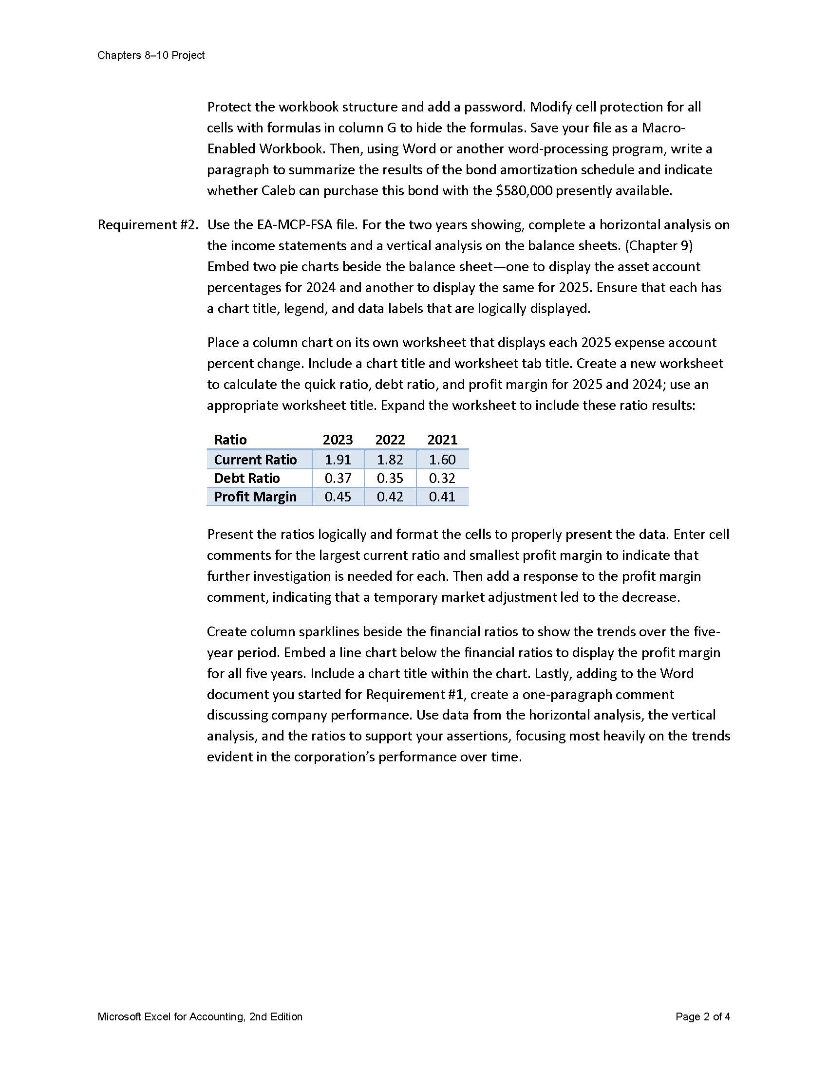
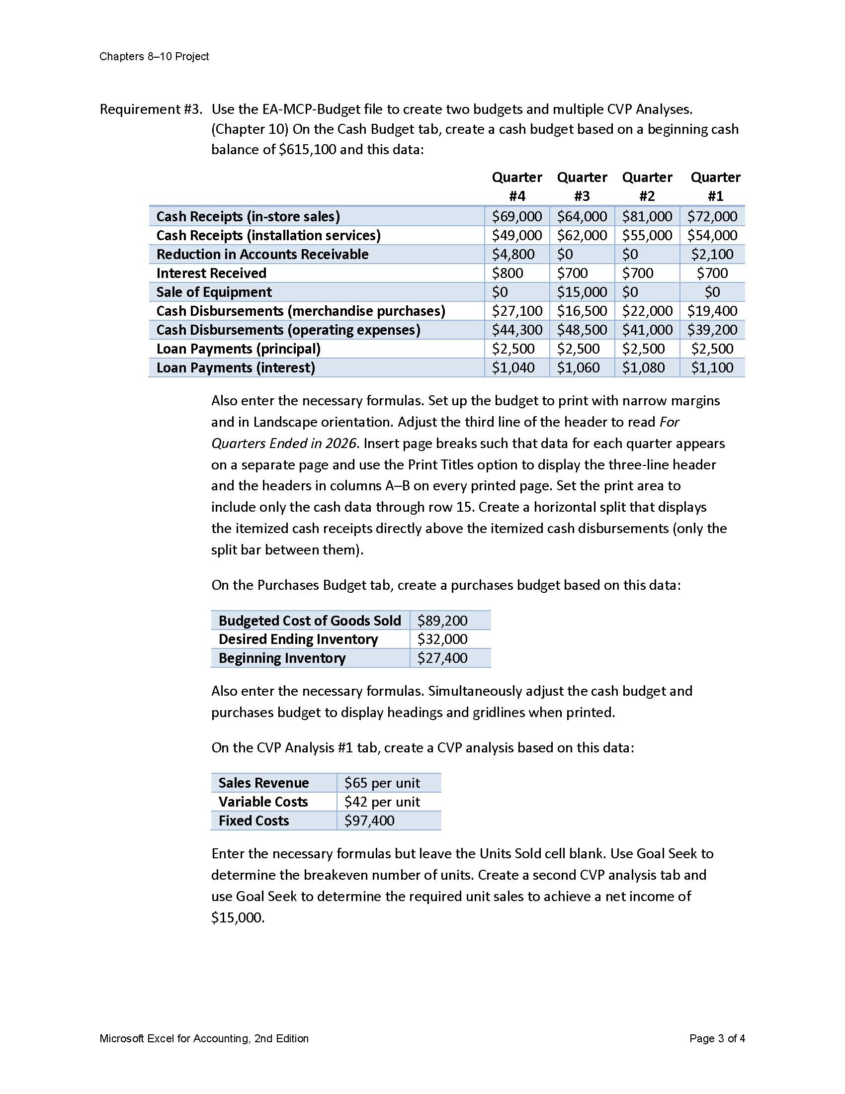
Excel for Accounting Multi-Chapter Project Chapters 8-10 In this project, you will use skills and procedures presented in Chapters 8-10 together as you analyze financial results for Offsides Corporation. Follow all instructions and use the approaches presented in the chapters to present the analysis in good form. Submit your work per your instructor's directions. Offsides Corporation manufactures hockey equipment and installs ice rinks in Boston, MA, and surrounding areas. The owner, Caleb Nelson, has built the business substantially since its inception five years ago. To maintain this growth, Caleb hires you as an outside consultant to help him make a few decisions. To begin, the business has accumulated significant cash reserves over its first three years, and Caleb is considering investing in a particular bond. He would like you to advise him as to whether the $580,000 of currently available cash is sufficient to purchase this bond. Next, Caleb would like to better understand whether operations have improved over the past few years. He wants you to perform a financial statement analysis, including an examination of key ratios, so you can advise him on the performance of the corporation. Finally, Caleb needs assistance in forecasting the company's performance over the next year by establishing both a cash budget and a purchases budget for 2026. He would also like to understand the unit sales necessary to break even and to earn profit at various levels over the next year. Project Requirements Requirement #1. Start a new file. Reduce the width of column A to 0.75 and the height of row 1 to 7.20. Enter the bond details in the range B2:C8. Include a centered header and appropriate titles. Enter the details for a bond with a $580,000 face value, a four-year life, semiannual interest payments, a contract interest rate of 9%, and an effective interest rate of 12%. The bond is issued on 1/1/26. (Hint: Values must be entered here so they can be used in subsequent formulas.) Enter bond calculations for the present value, future value, and payments in the range B10:C13. The future value will generate a result that matches the above figure; you complete this calculation to check your work. Create a bond amortization schedule beginning in cell B15 with the proper headers in row 15. (Chapter 8) Calculate totals for the appropriate columns. Assign an appropriate name to the worksheet tab. Record a macro that generates every formula in the worksheet after the bond details (in the range B2:C8) and dates have been entered. Run the macro to ensure it operates properly. Insert a text box in an appropriate location, add an appropriate name in it, and assign the macro to it. Microsoft Excel for Accounting Page 1 of 4 Chapters 8-10 Project Protect the workbook structure and add a password. Modify cell protection for all cells with formulas in column G to hide the formulas. Save your file as a Macro- Enabled Workbook. Then, using Word or another word-processing program, write a paragraph to summarize the results of the bond amortization schedule and indicate whether Caleb can purchase this bond with the $580,000 presently available. Requirement #2. Use the EA-MCP-FSA file. For the two years showing, complete a horizontal analysis on the income statements and a vertical analysis on the balance sheets. (Chapter 9) Embed two pie charts beside the balance sheet-one to display the asset account percentages for 2024 and another to display the same for 2025. Ensure that each has a chart title, legend, and data labels that are logically displayed. Place a column chart on its own worksheet that displays each 2025 expense account percent change. Include a chart title and worksheet tab title. Create a new worksheet to calculate the quick ratio, debt ratio, and profit margin for 2025 and 2024; use an appropriate worksheet title. Expand the worksheet to include these ratio results: Ratio Current Ratio Debt Ratio Profit Margin 2023 2022 2021 1.60 1.91 1.82 0.37 0.35 0.32 0.45 0.42 0.41 Present the ratios logically and format the cells to properly present the data. Enter cell comments for the largest current ratio and smallest profit margin to indicate that further investigation is needed for each. Then add a response to the profit margin comment, indicating that a temporary market adjustment led to the decrease. Create column sparklines beside the financial ratios to show the trends over the five- year period. Embed a line chart below the financial ratios to display the profit margin for all five years. Include a chart title within the chart. Lastly, adding to the Word document you started for Requirement #1, create a one-paragraph comment discussing company performance. Use data from the horizontal analysis, the vertical analysis, and the ratios to support your assertions, focusing most heavily on the trends evident in the corporation's performance over time. Microsoft Excel for Accounting, 2nd Edition Page 2 of 4 Chapters 8-10 Project Requirement #3. Use the EA-MCP-Budget file to create two budgets and multiple CVP Analyses. (Chapter 10) On the Cash Budget tab, create a cash budget based on a beginning cash balance of $615,100 and this data: Cash Receipts (in-store sales) Cash Receipts (installation services) Reduction in Accounts Receivable Interest Received Sale of Equipment Cash Disbursements (merchandise purchases) Cash Disbursements (operating expenses) Loan Payments (principal) Loan Payments (interest) Also enter the necessary formulas. Set up the budget to print with narrow margins and in Landscape orientation. Adjust the third line of the header to read For Quarters Ended in 2026. Insert page breaks such that data for each quarter appears on a separate page and use the Print Titles option to display the three-line header and the headers in columns A-B on every printed page. Set the print area to include only the cash data through row 15. Create a horizontal split that displays the itemized cash receipts directly above the itemized cash disbursements (only the split bar between them). On the Purchases Budget tab, create a purchases budget based on this data: Budgeted Cost of Goods Sold $89,200 Desired Ending Inventory $32,000 Beginning Inventory $27,400 Quarter Quarter Quarter Quarter #4 #3 #2 #1 $69,000 $64,000 $81,000 $72,000 $49,000 $62,000 $55,000 $54,000 $4,800 $0 $0 $2,100 $800 $700 $700 $0 $15,000 $0 $0 $27,100 $16,500 $22,000 $19,400 $44,300 $48,500 $41,000 $39,200 $2,500 $2,500 $2,500 $2,500 $1,040 $1,060 $1,080 $1,100 $700 Also enter the necessary formulas. Simultaneously adjust the cash budget and purchases budget to display headings and gridlines when printed. On the CVP Analysis #1 tab, create a CVP analysis based on this data: $65 per unit $42 per unit $97,400 Sales Revenue Variable Costs Fixed Costs Enter the necessary formulas but leave the Units Sold cell blank. Use Goal Seek to determine the breakeven number of units. Create a second CVP analysis tab and use Goal Seek to determine the required unit sales to achieve a net income of $15,000. Microsoft Excel for Accounting, 2nd Edition Page 3 of 4 Chapters 8-10 Project Create a third CVP analysis tab that assumes unit sales equal to those calculated in the second CVP analysis but that modifies other assumptions as follows: Assume fixed costs are the same as those in the first two CVP analyses and that they cannot change. Assume sales revenue per unit cannot exceed $66. Assume variable costs per unit cannot fall below $44. Assume the contribution margin must be less than or equal to 42% of sales revenue. Name each CVP tab appropriately. For each CVP analysis, freeze the three-line header at the top. Lastly, in your Word document, write a paragraph that summarizes the findings of the CVP analyses and that discusses the anticipated cash position based on the cash and purchases budgets you completed. Microsoft Excel for Accounting, 2nd Edition Page 4 of 4
Step by Step Solution
There are 3 Steps involved in it

Get step-by-step solutions from verified subject matter experts