EXCEL HELP

Read the step by step instruction (picture 1) and the case study (picture 2)

I have inputted some answers for the third picture and 4th picture but I am not sure if it is correct.

Needs to be redone.

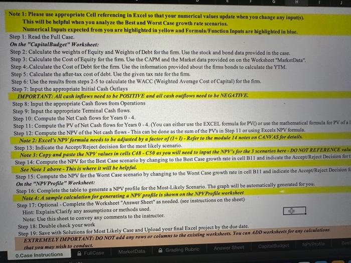
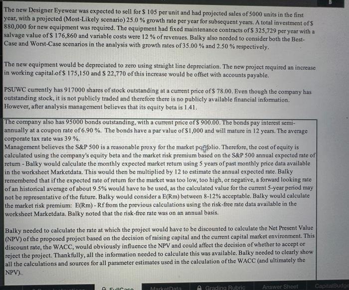
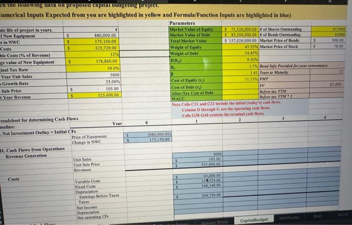
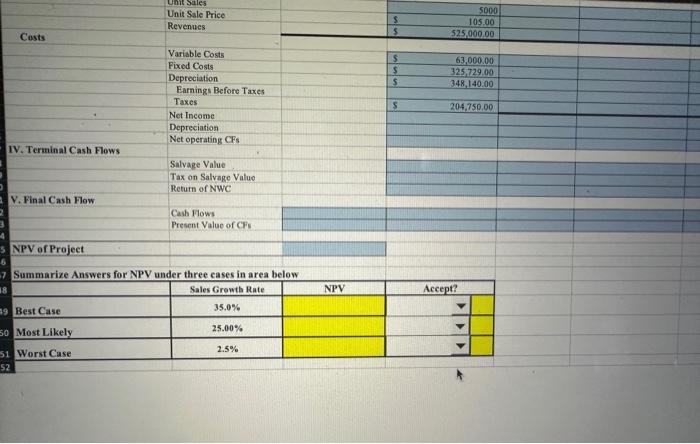
Note 1: Please use appropriate Cell referencing in Excel so that your numerical values update when you change any input(s). This will be helpful when you analyze the Best and Worst Case growth rate scenarios. Numerical Inputs expected from you are highlighted in yellow and Formula/Function Inputs are highlighted in blue. Step 1: Read the Full Case. On the "CapitalBudget" Worksheet: Step 2: Calculate the weights of Equity and Weights of Debt for the firm. Use the stock and bond data provided in the case. Step 3: Calculate the Cost of Equity for the firm. Use the CAPM and the Market data provided on on the Worksheet "MarketData". Step 4: Calculate the Cost of Debt for the firm. Use the information provided about the firms bonds to calculate the YTM. Step 5: Calculate the after-tax cost of debt. Use the given tax rate for the firm. Step 6: Use the results from steps 2-5 to calculate the WACC (Weighted Average Cost of Capital) for the fim. Step 7: Input the appropriate Initial Cash Outlays IMPORTANT: AII cash inflows need to be POSITIVE and all cash outflows need to be NEGATIVE: Step 8: Input the appropriate Cash flows from Operations Step 9: Input the appropriate Terminal Cash flows. Step 10: Compute the Net Cash flows for Years 04. Step 11: Compute the PV of Net Cash flows for Years 04. (You can either use the EXCEL formula for PVO or use the mathematical fomula for PV of a Step 12: Compute the NPV of the Net cash flows - This can be done as the sum of the PVs in Step 11 or using Excels NPV formula. Note 2: Excel's NPV formula needs to be adjusted by a factor of (1+1)-Refer to the module 14 notes on CANVAS for detaiks Step 13: Indicate the Accept/Reject decision for the most likely scenario. Note 3: Copy and paste the NPV values in cells C48 - C50 as you will need to input the NPV's for the 3 scenarios here - DO NOT REFERENCE wah Step 14: Compute the NPV for the Best Case scenario by changing to the Best Case growth rate in cell B1I and indicate the AcceptReject Decision for See Note I above - This is where it will be helpfil. Step 15: Compute the NPV for the Worst Case scenario by changing to the Worst Case growth rate in cell B11 and indicate the Accept/Reject Decision On the "NPVProfile" Worksheet: Step 16: Complete the table to generate a NPV profile for the Most-Likely Scenario. The graph will be automatically generated for you. Note 4: A sample calculation for generating a NPV profile is shown on the NPVProfile workshect Step 17: Optional - Complete the Worksheet "Answer Sheet" as needed. (see instructions on the sheet) Hint: Explain/Clarify any assumptions or methods used. Note: Use this sheet to convey any comments to the instructor. Step 18: Double check your work Step 19: Save with Solutions for Most Likely Case and Upload your final Excel project by the due date. EXTREMELY IMPORTANT: DO NOT add any rows or columns to the existing worksheets. You can ADD warksheets for any calculations The new Designer Eyewear was expected to sell for $105 per unit and had projected sales of 5000 units in the first year, with a projected (Most-Likely scenario) 25.0% growth rate per year for subsequent years. A total investment of $ 880,000 for new equipment was required. The equipment had fixed maintenance contracts of $325,729 per year with a salvage value of $176,860 and variable costs were 12% of revenues. Balky also needed to consider both the BestCase and Worst-Case scenarios in the analysis with growth rates of 35.00% and 2.50% respectively. The new equipment would be depreciated to zero using straight line depreciation. The new project required an increase in working capital.of $175,150 and $22,770 of this increase would be offset with accounts payable. PSUWC currently has 917000 shares of stock outstanding at a current price of $78.00. Even though the company has outstanding stock, it is not publicly traded and therefore there is no publicly available financial information. However, after analysis management believes that its equity beta is 1.41 . The company also has 95000 bonds outstanding, with a current price of $900.00. The bonds pay interest semiannually at a coupon rate of 6.90%. The bonds have a par value of $1,000 and will mature in 12 years. The average corporate tax rate was 39%. Management believes the S\&P 500 is a reasonable proxy for the market perfolio. Therefore, the cost of equity is calculated using the company's equity beta and the market risk premium based on the S\&P 500 annual expected rate of retum - Balky would calculate the monthly expected market retum using 5 years of past monthly price data available in the worksheet Marketdata. This would then be multiplied by 12 to estimate the annual expected rate. Balky remembered that if the expected rate of retum for the market was too low, too high, or negative, a forward looking rate of an historical average of about 9.5% would have to be used, as the calculated value for the current 5 -year period may not be representative of the future. Balky would consider a E(Rm) between 812% acceptable. Balky would calculate the market risk premium: E(Rm) - Rf from the previous calculations using the risk-free rate data available in the worksheet Marketdata. Balky noted that the risk-free rate was on an annual basis. Balky needed to calculate the rate at which the project would have to be discounted to calculate the Net Present Value (NPV) of the proposed project based on the decision of raising capital and the current capital market environment. This discount rate, the WACC, would obviously influence the NPV and could affect the decision of whether to accept or reject the project. Thankfully, all the information needed to calculate this was available. Balky needed to clearly show all the calculations and sources for all parameter estimates used in the calculation of the WACC (and ultimately the NPV). in the rono wing aara on proposea capitar Dugeung project. Unit Sale Price Revenues \begin{tabular}{|rr|} \hline 5 & 5000 \\ \hline 5 & 105,00 \\ \hline \end{tabular} Variable Costs Fixed Costs Depreciation Earnings Before Taxes Taxes Net Inceme Depreciation Net operating CFs Salvage Value Tax on Salvage Value Return of NWC Cash Flows Present Value of CFs NPV of Project Summarize Answers for NPV under three cases in area below \begin{tabular}{|l|c|c|c|} \hline Summarize Answers for NPV under three casesin area below & NPV & Accept? \\ \hline Best Case & Sales Growth Rate & & \\ \hline Most Likely & 35.0% & & \\ \hline Worst Case & 25.00% & & \\ \hline \end{tabular}