

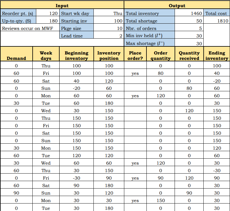
Question: EXplanation of below table = > The main input data that drive the simulation are the periodic review values s and S in the table.
EXplanation of below table
The main input data that drive the simulation are the periodic review values s and S in the
table. The initial values of s and S used to start iterative simulations are as follows:
Q Economic order quantity
s Maximum demand of an order period based on historical data
S s Q
The output results of the simulation are then used to search for a lower cost policy, and, if
found, the new s S values are entered in the table and the simulation is run anew for the
same demand stream in the first column. The procedure is repeated until no better policy
can be found, as will be explained below.
The remaining input data provide start week day Thursday starting inventory
package size and lead time days The start week day is used to enhance readability,
and all orders must be rounded up to multiples of the package size.
The cost data includes the fixed ordering cost $order the holding cost $unitday
and the stockout cost $unitday
The spreadsheet calculations are based on the following ordering policy and simulation
formulas:
Ordering policy:
On a review day, if inventory position s order S inventory position else do not
order.
Inventory position reviewed on Mondays, Wednesdays and Fridays.
Order is placed at the end of the day and remains outstanding throughout the lead
time.
Filled order is received at the end of the day.
All unfilled demand is backordered no lost sales
Simulation formulas day i:
Beginning inventoryi Ending inventoryi
Ending inventoryi Beginning inventoryi Received orderi Demandi
Inventory positioni Beginning inventoryi On orderi
A summary output of the simulation includes: total inventory, total shortage, number of orders placed, minimum positive ending inventory and maximum shortage The output data also include the total inventory cost per day comprised of the sum of order setup cost, holding cost, and shortage cost. This cost function evaluates different periodic review policies.
Local Search Algorithm EXplanation
The search starts with an initial review policy s s Q defined previously. The values used in Table are s and Q giving S Define s S as the best review policy so far found with cost C and quantities and
The idea is to look for a better review policy in the neighborhood of s S based on two steps: Step Fixed Q
a Set and and run the simulation for the new policy s S If it
yields a lower cost, update s Ss S and repeat a Else go to b
b Set and and run the simulation for the new policy s S If it
yields a lower cost, update s Ss S and repeat a Else, no better solution can be found for fixed Q Go to Step
Step Variable Q: Let rmin
a Set yielding and run the simulation for the new policy s
S If it yields a lower cost, update s Ss S and go to Step a Else go to b
b Set yielding and run the simulation for the new policy s
S If it yields a lower cost, update s Ss S and go to Step a Else, no better solution can be found for variable Q Stop.
In Step Q is kept fixed by changing increasing or decreasing s and S by equal amounts. Step a increases both s and S in an attempt to eliminate the shortage and Step b tries to bring the minimum ending inventory to zero by decreasing both s and S If Step fails to produce a better solution for a fixed Q Step with a similar line of reasoning as in Step varies the value of Q by changing s and S one at a time. When Step cannot produce a better review policy, the search ends with the last s and S values providing the best heuristic solution.
Implementation
Kroger reports that developed model was implemented in in all the pharmacies in the United States. It has resulted in appreciable reduction in shortages and increase in revenues. The increase in revenues is estimated at $ million, and was coupled with a reduction in inventory of about $ million.Plans are underway to extend the model to other store departments. In particular, perishable products could benefit from a similar inventory control application with the goal of eliminating losses resulting from spoilage.
QUESTION
Develop a spreadsheet simulation and apply the local search algorithm to find the s and S values that Kroger should use in their inventory policy. Use the initial values given in Table
Step by Step Solution
There are 3 Steps involved in it
1 Expert Approved Answer
Step: 1 Unlock

Question Has Been Solved by an Expert!
Get step-by-step solutions from verified subject matter experts
Step: 2 Unlock
Step: 3 Unlock