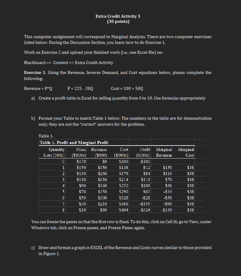
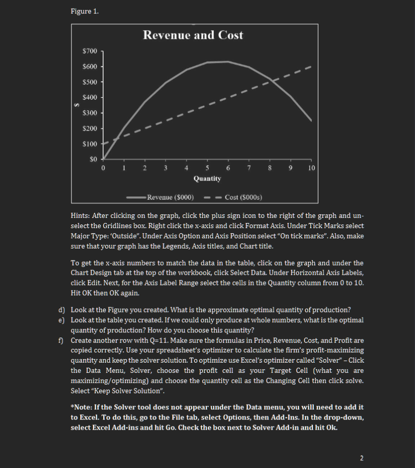
Extra Credit Activity 3 (30 points) This computer assignment will correspond to Marginal Analysis. There are two computer exercises listed below. During the Discussion Section, you learn how to do Exercise 1. Work on Exercise 2 and upload your finished work (i.e., one Excel file) on: Blackboard => Content => Extra Credit Activity Exercise 1. Using the Revenue, Inverse Demand, and Cost equations below, please complete the following: Revenue = P*Q P =225 - 20Q Cost = 100 + 50Q a) Create a profit table in Excel for selling quantity from 0 to 10. Use formulas appropriately b) Format your Table to match Table 1 below. The numbers in the table are for demonstration only; they are not the "correct" answers for the problem. Table 1. Table 1. Profit and Marginal Profit Quantity Price Revenue Cost Profit Marginal Marginal Lots (000s) ($0003) $000) ($000s) (SOODs Revenue Cost $170 50 $100 $100 $150 $150 $138 $12 $150 $38 2 $130 $260 $176 $84 $110 $38 3 $110 $330 $214 $116 $70 $38 4 $90 $360 $252 $108 $30 $38 5 $70 $350 $290 560 -$10 $38 6 $50 $300 $328 -$28 -$50 $38 7 $30 $210 $365 -$156 -$90 $38 $10 $80 $404 -$324 -$130 $38 You can freeze the panes so that the first row is fixed. To do this, click on Cell 16, go to View, under Windows tab, click on Freeze panes, and Freeze Panes again. c) Draw and format a graph in EXCEL of the Revenue and Costs curves similar to those provided in Figure 1.Figure 1. Revenue and Cost Quantity Revenue ($000) T Hints: After clicking on the graph, click the plus sign icon to the right of the graph and un- select the Gridlines box. Right click the x-axis and click Format Axis. Under Tick Marks select Major Type: 'Outside\". Under Axis Option and Axis Position select \"On tick marks". Also, make sure that your graph has the Legends, Axis titles, and Chart title. To get the x-axis numbers to match the data in the table, click on the graph and under the Chart Design tab at the top of the workbook, click Select Data. Under Horizontal Axis Labels, click Edit. Next, for the Axis Label Range select the cells in the Quantity column from 0 to 10. Hit OK then OK again. Look at the Figure you created. What is the approximate optimal quantity of production? Look at the table you created. If we could only produce at whole numbers, what is the optimal gquantity of production? How do you choose this guantity? Create another row with Q=11. Make sure the formulas in Price, Revenue, Cost, and Profit are copied correctly. Use your spreadsheet's optimizer to calculate the firm's profit-maximizing guantity and keep the solver solution. To optimize use Excel's optimizer called \"Solver\" - Click the Data Menu, Solver, choose the profit cell as your Target Cell (what you are maximizing/optimizing) and choose the quantity cell as the Changing Cell then click solve. Select \"Keep Solver Solution\". *Note: If the Solver tool does not appear under the Data menu, you will need to add it to Excel. To do this, go to the File tab, select Options, then Add-Ins. In the drop-down, select Excel Add-ins and hit Go. Check the box next to Solver Add-in and hit Ok. Exercise 2. (30 points) A manufacture of spare parts faces the demand curve, P = 750 - 4() and produces output according to the cost function, Cost = 12,000 + 200Q + 0.5Q:. Provide expressions for revenue, cost, profit, marginal revenue and marginal cost. To enter (2 use * i.e. Q*2. a) (10 points) Create a profit table in Excel for selling quantity from Oto 100. Use formulas appropriately. Format your Table to match Table 1 in Question 1. Freeze the first row. b} (10 points) Draw and format a graph in EXCEL of the Revenue, Cost, and Profit curves similar to those provided in Figure 1. Make sure yvour horizontal axis is from 0 to 100, and that your graph is properly labeled (Legends, Axis titles, and Chart title) = 2 points for horizontal axis, 1 point for horizontal label, 1 point for vertical label, 1 point for chart title, 3 points for legends, 3 points for Revenue graph, 3 points for Cost graph, 3 peints for Profit graph (5 points: 2 points for the right answer, 3 points for the explanation) Look at the table you created. If we could only produce at whole numbers, what is the optimal quantity of production? Why? (5 points) Create another row with Q=101. Make sure the formulas in Price, Revenue, Cost, and Profit are copied correctly. Use Solver to calculate the firm's profit-maximizing quantity and keep the solver solution