

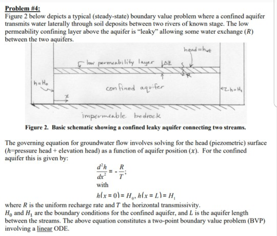
Question: Figure 2 below depicts a typical (steady-state) boundary value problem where a confined aquifer transmits water laterally through soil deposits between two rivers of known
Figure 2 below depicts a typical (steady-state) boundary value problem where a confined aquifer transmits water laterally through soil deposits between two rivers of known stage.
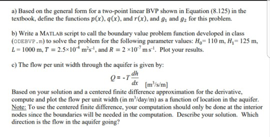
(Please solve all parts and include Matlab code, thank you)
ODEBVP.m funtion provided here:
function z = ODEBVP(p,q,r,a,b,ga,gb,N)
% A program to solve the two point boundary value problem
% y''=p(x)y'+q(x)y+r(x), a % y(a)=g1, y(b)=g2 % Input % p, q, r: coefficient functions % a, b: the end-points of the interval % ga, gb: the prescribed function values at the end-points % N: number of sub-intervals % Output % z = [ xx yy ]: xx is an (N+1) column vector of the node points % yy is an (N+1) column vecotr of the solution values % A sample call would be % z=ODEBVP('p','q','r',a,b,ga,gb,100) % The user must provide m-files to define the functions p, q and r. % % Other MATLAB program called: tridiag.m % % Initialization N1 = N+1; h = (b-a)/N; h2 = h*h; xx = linspace(a,b,N1)'; yy = zeros(N1,1); yy(1) = ga; yy(N1) = gb; % Define the sub-diagonal avec, main diagonal bvec, superdiagonal cvec pp(2:N) = feval(p,xx(2:N)); avec(2:N-1) = -1-(h/2)*pp(3:N); bvec(1:N-1) = 2+h2*feval(q,xx(2:N)); cvec(1:N-2) = -1+(h/2)*pp(2:N-1); % Define the right hand side vector fvec fvec(1:N-1) = -h2*feval(r,xx(2:N)); fvec(1) = fvec(1)+(1+h*pp(2)/2)*ga; fvec(N-1) = fvec(N-1)+(1-h*pp(N)/2)*gb; % Solve the tridiagonal system yy(2:N) = tridiag(avec,bvec,cvec,fvec,N-1,0); z = [xx'; yy']';
Step by Step Solution
There are 3 Steps involved in it

Get step-by-step solutions from verified subject matter experts