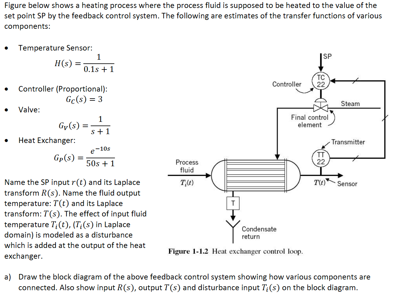
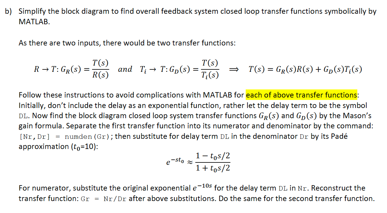
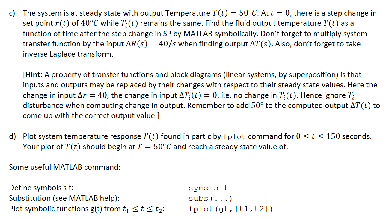
Figure below shows a heating process where the process fluid is supposed to be heated to the value of the set point SP by the feedback control system. The following are estimates of the transfer functions of various components: Temperature Sensor: 1 H(s) = 0 15+1 Controller Steam 1 Controller (Proportional): Gc(s) = 3 Valve: Gy(s) = -1 Heat Exchanger: Gp(s) = 50s +1 Final control element S + 1 Transmitter e-10s Process fluid T;(t) T(t) Sensor Name the SP input r(t) and its Laplace transform R(s). Name the fluid output temperature: T(t) and its Laplace transform:T(s). The effect of input fluid temperature Ti(t), (Ti(s) in Laplace domain) is modeled as a disturbance which is added at the output of the heat exchanger. Condensate return Figure 1-1.2 Heat exchanger control loop. a) Draw the block diagram of the above feedback control system showing how various components are connected. Also show input R(s), output T(s) and disturbance input Ti(s) on the block diagram. b) Simplify the block diagram to find overall feedback system closed loop transfer functions symbolically by MATLAB. As there are two inputs, there would be two transfer functions: T(S) R T:GR(S) = Dio and Ti T:GD(S) = T = T(s) = Gr(s)R(s) + Gp(s)T;(s) Follow these instructions to avoid complications with MATLAB for each of above transfer functions: Initially, don't include the delay as an exponential function, rather let the delay term to be the symbol DL. Now find the block diagram closed loop system transfer functions Gr(s) and GD(s) by the Mason's gain formula. Separate the first transfer function into its numerator and denominator by the command: [Nr, Dr] = numden (Gr); then substitute for delay term DL in the denominator Dr by its Pad approximation (to=10): e-sto - 1- tos/2 1+ tos/2 For numerator, substitute the original exponential e-10s for the delay term DL in Nr. Reconstruct the transfer function: Gr = Nr/Dr after above substitutions. Do the same for the second transfer function. c) The system is at steady state with output Temperature T(t) = 50C. At t = 0, there is a step change in set point r(t) of 40C while Ti(t) remains the same. Find the fluid output temperature T(t) as a function of time after the step change in SP by MATLAB symbolically. Don't forget to multiply system transfer function by the input AR(s) = 40/s when finding output AT(s). Also, don't forget to take inverse Laplace transform. [Hint: A property of transfer functions and block diagrams (linear systems, by superposition) is that inputs and outputs may be replaced by their changes with respect to their steady state values. Here the change in input Ar = 40, the change in input ATi(t) = 0, i.e. no change in Ti(t). Hence ignore Ti disturbance when computing change in output. Remember to add 50 to the computed output AT(t) to come up with the correct output value.] d) Plot system temperature response T(t) found in part c by fplot command for 0 st = 150 seconds. Your plot of T(t) should begin at T = 50C and reach a steady state value of. Some useful MATLAB command: Define symbols st: Substitution (see MATLAB help): Plot symbolic functions g(t) from t1 st s tz: syms St subs (...) fplot (gt, [t1, t2]). Figure below shows a heating process where the process fluid is supposed to be heated to the value of the set point SP by the feedback control system. The following are estimates of the transfer functions of various components: Temperature Sensor: 1 H(s) = 0 15+1 Controller Steam 1 Controller (Proportional): Gc(s) = 3 Valve: Gy(s) = -1 Heat Exchanger: Gp(s) = 50s +1 Final control element S + 1 Transmitter e-10s Process fluid T;(t) T(t) Sensor Name the SP input r(t) and its Laplace transform R(s). Name the fluid output temperature: T(t) and its Laplace transform:T(s). The effect of input fluid temperature Ti(t), (Ti(s) in Laplace domain) is modeled as a disturbance which is added at the output of the heat exchanger. Condensate return Figure 1-1.2 Heat exchanger control loop. a) Draw the block diagram of the above feedback control system showing how various components are connected. Also show input R(s), output T(s) and disturbance input Ti(s) on the block diagram. b) Simplify the block diagram to find overall feedback system closed loop transfer functions symbolically by MATLAB. As there are two inputs, there would be two transfer functions: T(S) R T:GR(S) = Dio and Ti T:GD(S) = T = T(s) = Gr(s)R(s) + Gp(s)T;(s) Follow these instructions to avoid complications with MATLAB for each of above transfer functions: Initially, don't include the delay as an exponential function, rather let the delay term to be the symbol DL. Now find the block diagram closed loop system transfer functions Gr(s) and GD(s) by the Mason's gain formula. Separate the first transfer function into its numerator and denominator by the command: [Nr, Dr] = numden (Gr); then substitute for delay term DL in the denominator Dr by its Pad approximation (to=10): e-sto - 1- tos/2 1+ tos/2 For numerator, substitute the original exponential e-10s for the delay term DL in Nr. Reconstruct the transfer function: Gr = Nr/Dr after above substitutions. Do the same for the second transfer function. c) The system is at steady state with output Temperature T(t) = 50C. At t = 0, there is a step change in set point r(t) of 40C while Ti(t) remains the same. Find the fluid output temperature T(t) as a function of time after the step change in SP by MATLAB symbolically. Don't forget to multiply system transfer function by the input AR(s) = 40/s when finding output AT(s). Also, don't forget to take inverse Laplace transform. [Hint: A property of transfer functions and block diagrams (linear systems, by superposition) is that inputs and outputs may be replaced by their changes with respect to their steady state values. Here the change in input Ar = 40, the change in input ATi(t) = 0, i.e. no change in Ti(t). Hence ignore Ti disturbance when computing change in output. Remember to add 50 to the computed output AT(t) to come up with the correct output value.] d) Plot system temperature response T(t) found in part c by fplot command for 0 st = 150 seconds. Your plot of T(t) should begin at T = 50C and reach a steady state value of. Some useful MATLAB command: Define symbols st: Substitution (see MATLAB help): Plot symbolic functions g(t) from t1 st s tz: syms St subs (...) fplot (gt, [t1, t2])