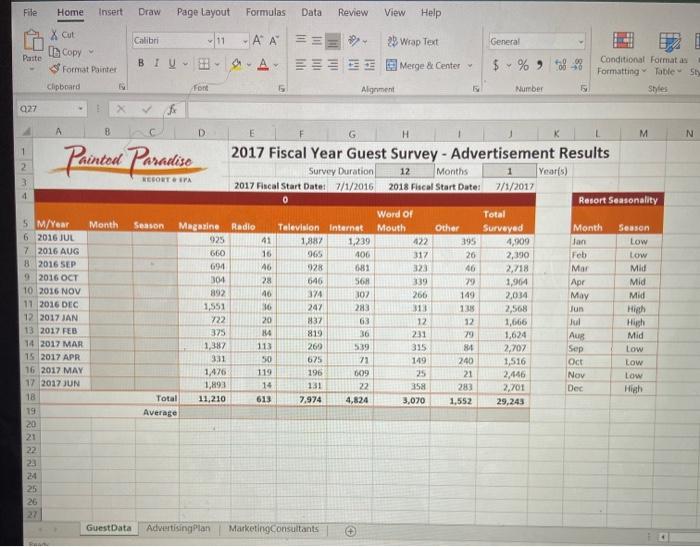
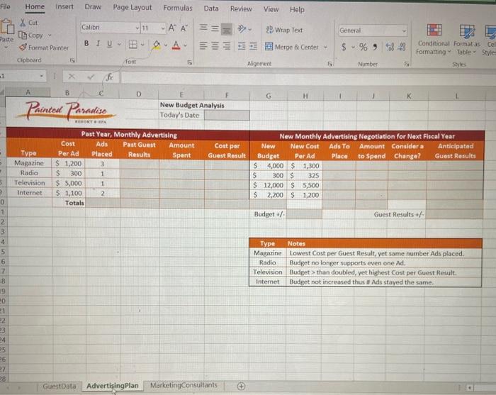
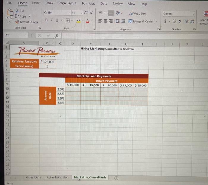
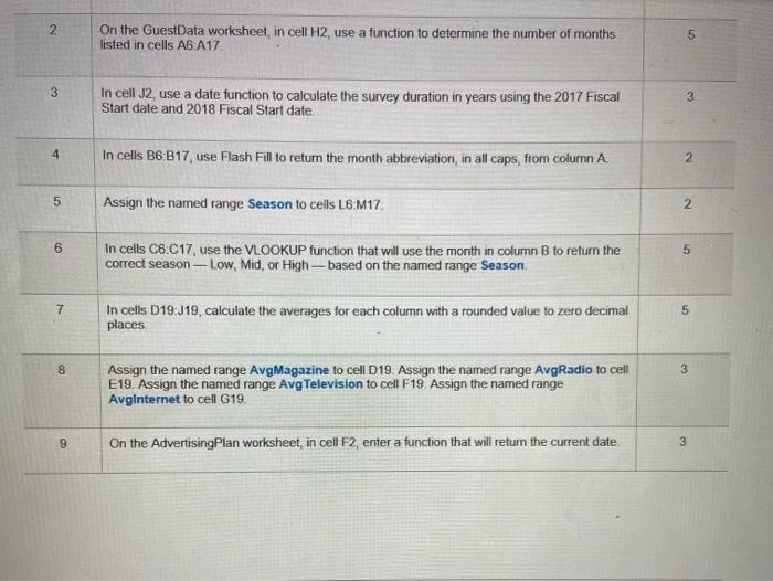
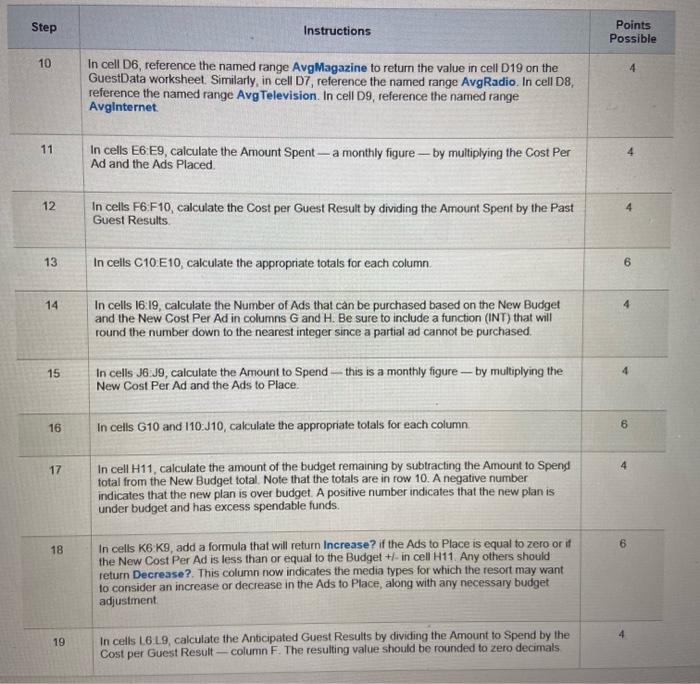
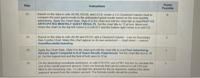
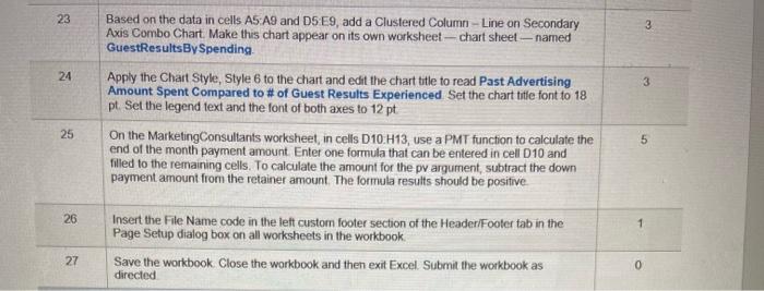
File Home Insert Draw Page Layout Formulas Data Review View Help Calibri 2 Wrap Text General x cut A copy Format Painter Clipboard 11AA == SA Paste BIU Merge & Center $ % *38% Conditional Formatan Formatting Tables Shes font Algement Number 927 8 N 1 2 Painted Paradise 965 100 5 M/Year Month 6 2016 JUL 7. 2016 AUG 8 2016 SEP 9 2016 OCT 10 2016 NOV 11 2016 DEC 12 2017 JAN 13 2017 FEB 14 2017 MAR 15 2017 APR 16 2017 MAY 17 2017 JUN 18 19 20 21 22 D G H M 2017 Fiscal Year Guest Survey - Advertisement Results Survey Duration 12 Months Year(s) RESORT SPA 2017 Fiscal Start Dates 7/1/2016 2018 Fiscal Start Date: 7/1/2017 Resort Seasonality Word of Total Season Magazine Radio Television Internet Mouth Other Surveyed Month Season 925 41 1,887 1,239 422 395 4,909 Jan Low 660 16 317 26 2,390 Feb Low 694 46 928 681 323 16 2,718 Mar Mid 304 28 646 568 339 29 1,964 Apr Mid 892 40 374 307 266 149 2,034 May Mid 1,551 36 247 283 313 135 2,568 Jun High 722 20 837 63 12 12 1,666 Jul 375 14 819 36 231 29 1,624 Aug Mid 1,387 113 269 5.39 335 81 2,707 Sep Low 50 625 71 149 240 1,516 loct Low 1.476 119 196 0679 25 21 2.446 Nov Low 1,893 14 131 22 283 2,701 Dec Total 11,210 613 7,974 4,824 3,070 1,552 29,243 Average 331 25 26 GuestData Advertising Plan Marketing Consultants File Home Insert Draw Page Layout Formulas Data Review View Help Calibri Xcut Copy Paste Format Painter General 11AA BIU-BAA 2 Wrap Text Merge & Center $ Conditional Formatastel Formatting Table Style Styles Clipboard Font 5 Alignment Number -1 A G H Painted Paradiso B D New Budget Analysis Today's Date MEKTET Past Year, Monthly Advertising Cost Ads Past Guest Amount Cost per Per Ad Placed Results Spent Guest Result $ 1,200 3 S 300 1 $ 5,000 1 $ 1,100 2 Totals Type Magazine Radio Television Internet New Monthly Advertising Negotiation for Next Fiscal Year New New Cost Ads To Amount Considera Anticipated Budget Per Ad Place to Spend Change? Guest Results S 4,000 $1,300 $ 300 S 325 $ 12,000 $5,500 $ 2,200 $1,200 8 Budget/ Guest Results + Type Notes Magazine Lowest Cost per Guest Result, vet same number Ads placed Radio Budget no longer supports even one Ad Television Budget >than doubled, yet highest Cost per Guest Result. Intemet Budget not increased thus 11 Ads stayed the same. 0 1 2 3 4 5 6 17 8 19 20 21 22 3 24 25 26 27 28 GuestData Advertising Plan Marketing Consultants File Home Insert Draw Page Layout Formulas Data Review View Help X Cut [Copy Calibri 11 A A General HT Paste illl!!! 2 Wrap Text * Merge & Center BIO Format Painter $ % 8-98 Condit Format Clipboard 15 Font Alignment Number A1 fi B D H K 1 Painted Paradise Hiring Marketing Consultants Analysis 2 3 4 Retainer Amount $ 125,000 Term (Years) 5 Monthly Loan Payments Down Payment $ 10,000 $ 15,000 $20,000 $25,000 $30,000 Annual Rate 2.0% 2.5% 3.0% 3.5% 5 6 7 8 9 10 11 12 13 14 15 16 17 18 19 20 21 22 23 24 25 26 27 28 29 GuestData Advertising Plan Marketing Consultants Ready 2 On the GuestData worksheet, in cell H2, use a function to determine the number of months listed in cells A6 A17 5 3 In cell 32, use a date function to calculate the survey duration in years using the 2017 Fiscal Start date and 2018 Fiscal Start date. 3 4 In cells B6 B17, use Flash Fill to return the month abbreviation, in all caps, from column A. 2 5 Assign the named range Season to cells L6:M17 2. 6 5 In cells C6 C17, use the VLOOKUP function that will use the month in column B to return the correct season - Low, Mid, or High-based on the named range Season 7 on In cells D19:19, calculate the averages for each column with a rounded value to zero decimal places 8 3 Assign the named range AvgMagazine to cell D19. Assign the named range Avg Radio to cell E19. Assign the named range Avg Television to cell F19 Assign the named range Avginternet to cell G19. 9 On the Advertising Plan worksheet, in cell F2, enter a function that will return the current date. 3 Step Instructions Points Possible 10 In cell D6, reference the named range Avg Magazine to return the value in cell D19 on the GuestData worksheet. Similarly, in cell D7, reference the named range Avg Radio. In cell D8, reference the named range Avg Television. In cell D9, reference the named range Avginternet 11 4 In cells E6 E9, calculate the Amount Spent - a monthly figure --- by multiplying the Cost Per Ad and the Ads Placed 12 4 In cells F6 F10, calculate the cost per Guest Result by dividing the Amount Spent by the Past Guest Results 13 In cells C10 E10, calculate the appropriate totals for each column 6 14 4 In cells 16:19, calculate the Number of Ads that can be purchased based on the New Budget and the New Cost Per Ad in columns G and H. Be sure to include a function (INT) that will round the number down to the nearest integer since a partial ad cannot be purchased. 15 In cells 36:39, calculate the amount to Spend -- this is a monthly figure - by multiplying the New Cost Per Ad and the Ads to Place. 16 In cells G10 and 110:10, calculate the appropriate totals for each column 4 17 In cell H11, calculate the amount of the budget remaining by subtracting the Amount to Spend total from the New Budget total. Note that the totals are in row 10. A negative number indicates that the new plan is over budget. A positive number indicates that the new plan is under budget and has excess spendable funds. 6 18 In cells K6 K9, add a formula that will return Increase? if the Ads to place is equal to zero or it the New Cost Per Ad is less than or equal to the Budget +- in cell H11 Any others should return Decrease?. This column now indicates the media types for which the resort may want to consider an increase or decrease in the Ads to Place, along with any necessary budget adjustment 4 19 In cells 16 L9, calculate the Anticipated Guest Results by dividing the Amount to Spend by the Cost per Guest Result -- column F. The resulting value should be rounded to zero decimals 20 In cell L.10, calculate the appropriate total for Anticipated Guest Results 21 4 In cell L11, calculate the amount of anticipated guest results compared to the past by subtracting the Past Guest Results total from the Anticipated Guest Results total. Note that the totals are in row 10. A negative number indicates an anticipated decrease in Guest Results. A positive number indicates an anticipated increase in Guest Results Step Instructions Points Possible 22 6 Based on the data in cells A5 A9, D5 D9, and L5L9, create a 3-D Clustered Column chart to compare the past guest results to the anticipated guest results based on the new monthly advertising Apply the Chart Style, Style 6 to the chart and edit the chart title to read PASTVS. ANTICIPATED MONTHLY GUEST RESULTS Set the chart title to 12 pt font. Move and resize the chart so the top left comer is in cell A11 and the bottom right comer is in cell F22. 23 3 24 3 Based on the data in cells A5 A9 and 5 E9, add a Clustered Column-Line on Secondary Axis Combo Chart Make this chart appear on its own worksheet - chart sheet-named GuestResultsBy Spending Apply the Chart Style, Style 6 to the chart and edit the chart title to read Past Advertising Amount Spent compared to # of Guest Results Experienced Set the chart title font to 18 pt Set the legend text and the font of both axes to 12 pt On the Marketing Consultants worksheet, in cells D10 H13, use a PMT function to calculate the end of the month payment amount. Enter one formula that can be entered in cell D10 and filled to the remaining cells To calculate the amount for the pv argument subtract the down payment amount from the retainer amount. The formula results should be positive 25 5 23 3 24 3 Based on the data in cells AS:A9 and DS E9, add a Clustered Column - Line on Secondary Axis Combo Chart Make this chart appear on its own worksheet - chart sheet - named GuestResultsBy Spending Apply the Chart Style, Style 6 to the chart and edit the chart title to read Past Advertising Amount Spent Compared to # of Guest Results Experienced Set the chart title font to 18 pt. Set the legend text and the font of both axes to 12 pt On the Marketing Consultants worksheet, in cells D10 H13, use a PMT function to calculate the end of the month payment amount Enter one formula that can be entered in cell D10 and filled to the remaining cells. To calculate the amount for the pv argument, subtract the down payment amount from the retainer amount. The formula results should be positive 25 5 26 1 Insert the File Name code in the left custom footer section of the Header/Footer tab in the Page Setup dialog box on all worksheets in the workbook Save the workbook. Close the workbook and then exit Excel Submit the workbook as directed 27 0 File Home Insert Draw Page Layout Formulas Data Review View Help Calibri 2 Wrap Text General x cut A copy Format Painter Clipboard 11AA == SA Paste BIU Merge & Center $ % *38% Conditional Formatan Formatting Tables Shes font Algement Number 927 8 N 1 2 Painted Paradise 965 100 5 M/Year Month 6 2016 JUL 7. 2016 AUG 8 2016 SEP 9 2016 OCT 10 2016 NOV 11 2016 DEC 12 2017 JAN 13 2017 FEB 14 2017 MAR 15 2017 APR 16 2017 MAY 17 2017 JUN 18 19 20 21 22 D G H M 2017 Fiscal Year Guest Survey - Advertisement Results Survey Duration 12 Months Year(s) RESORT SPA 2017 Fiscal Start Dates 7/1/2016 2018 Fiscal Start Date: 7/1/2017 Resort Seasonality Word of Total Season Magazine Radio Television Internet Mouth Other Surveyed Month Season 925 41 1,887 1,239 422 395 4,909 Jan Low 660 16 317 26 2,390 Feb Low 694 46 928 681 323 16 2,718 Mar Mid 304 28 646 568 339 29 1,964 Apr Mid 892 40 374 307 266 149 2,034 May Mid 1,551 36 247 283 313 135 2,568 Jun High 722 20 837 63 12 12 1,666 Jul 375 14 819 36 231 29 1,624 Aug Mid 1,387 113 269 5.39 335 81 2,707 Sep Low 50 625 71 149 240 1,516 loct Low 1.476 119 196 0679 25 21 2.446 Nov Low 1,893 14 131 22 283 2,701 Dec Total 11,210 613 7,974 4,824 3,070 1,552 29,243 Average 331 25 26 GuestData Advertising Plan Marketing Consultants File Home Insert Draw Page Layout Formulas Data Review View Help Calibri Xcut Copy Paste Format Painter General 11AA BIU-BAA 2 Wrap Text Merge & Center $ Conditional Formatastel Formatting Table Style Styles Clipboard Font 5 Alignment Number -1 A G H Painted Paradiso B D New Budget Analysis Today's Date MEKTET Past Year, Monthly Advertising Cost Ads Past Guest Amount Cost per Per Ad Placed Results Spent Guest Result $ 1,200 3 S 300 1 $ 5,000 1 $ 1,100 2 Totals Type Magazine Radio Television Internet New Monthly Advertising Negotiation for Next Fiscal Year New New Cost Ads To Amount Considera Anticipated Budget Per Ad Place to Spend Change? Guest Results S 4,000 $1,300 $ 300 S 325 $ 12,000 $5,500 $ 2,200 $1,200 8 Budget/ Guest Results + Type Notes Magazine Lowest Cost per Guest Result, vet same number Ads placed Radio Budget no longer supports even one Ad Television Budget >than doubled, yet highest Cost per Guest Result. Intemet Budget not increased thus 11 Ads stayed the same. 0 1 2 3 4 5 6 17 8 19 20 21 22 3 24 25 26 27 28 GuestData Advertising Plan Marketing Consultants File Home Insert Draw Page Layout Formulas Data Review View Help X Cut [Copy Calibri 11 A A General HT Paste illl!!! 2 Wrap Text * Merge & Center BIO Format Painter $ % 8-98 Condit Format Clipboard 15 Font Alignment Number A1 fi B D H K 1 Painted Paradise Hiring Marketing Consultants Analysis 2 3 4 Retainer Amount $ 125,000 Term (Years) 5 Monthly Loan Payments Down Payment $ 10,000 $ 15,000 $20,000 $25,000 $30,000 Annual Rate 2.0% 2.5% 3.0% 3.5% 5 6 7 8 9 10 11 12 13 14 15 16 17 18 19 20 21 22 23 24 25 26 27 28 29 GuestData Advertising Plan Marketing Consultants Ready 2 On the GuestData worksheet, in cell H2, use a function to determine the number of months listed in cells A6 A17 5 3 In cell 32, use a date function to calculate the survey duration in years using the 2017 Fiscal Start date and 2018 Fiscal Start date. 3 4 In cells B6 B17, use Flash Fill to return the month abbreviation, in all caps, from column A. 2 5 Assign the named range Season to cells L6:M17 2. 6 5 In cells C6 C17, use the VLOOKUP function that will use the month in column B to return the correct season - Low, Mid, or High-based on the named range Season 7 on In cells D19:19, calculate the averages for each column with a rounded value to zero decimal places 8 3 Assign the named range AvgMagazine to cell D19. Assign the named range Avg Radio to cell E19. Assign the named range Avg Television to cell F19 Assign the named range Avginternet to cell G19. 9 On the Advertising Plan worksheet, in cell F2, enter a function that will return the current date. 3 Step Instructions Points Possible 10 In cell D6, reference the named range Avg Magazine to return the value in cell D19 on the GuestData worksheet. Similarly, in cell D7, reference the named range Avg Radio. In cell D8, reference the named range Avg Television. In cell D9, reference the named range Avginternet 11 4 In cells E6 E9, calculate the Amount Spent - a monthly figure --- by multiplying the Cost Per Ad and the Ads Placed 12 4 In cells F6 F10, calculate the cost per Guest Result by dividing the Amount Spent by the Past Guest Results 13 In cells C10 E10, calculate the appropriate totals for each column 6 14 4 In cells 16:19, calculate the Number of Ads that can be purchased based on the New Budget and the New Cost Per Ad in columns G and H. Be sure to include a function (INT) that will round the number down to the nearest integer since a partial ad cannot be purchased. 15 In cells 36:39, calculate the amount to Spend -- this is a monthly figure - by multiplying the New Cost Per Ad and the Ads to Place. 16 In cells G10 and 110:10, calculate the appropriate totals for each column 4 17 In cell H11, calculate the amount of the budget remaining by subtracting the Amount to Spend total from the New Budget total. Note that the totals are in row 10. A negative number indicates that the new plan is over budget. A positive number indicates that the new plan is under budget and has excess spendable funds. 6 18 In cells K6 K9, add a formula that will return Increase? if the Ads to place is equal to zero or it the New Cost Per Ad is less than or equal to the Budget +- in cell H11 Any others should return Decrease?. This column now indicates the media types for which the resort may want to consider an increase or decrease in the Ads to Place, along with any necessary budget adjustment 4 19 In cells 16 L9, calculate the Anticipated Guest Results by dividing the Amount to Spend by the Cost per Guest Result -- column F. The resulting value should be rounded to zero decimals 20 In cell L.10, calculate the appropriate total for Anticipated Guest Results 21 4 In cell L11, calculate the amount of anticipated guest results compared to the past by subtracting the Past Guest Results total from the Anticipated Guest Results total. Note that the totals are in row 10. A negative number indicates an anticipated decrease in Guest Results. A positive number indicates an anticipated increase in Guest Results Step Instructions Points Possible 22 6 Based on the data in cells A5 A9, D5 D9, and L5L9, create a 3-D Clustered Column chart to compare the past guest results to the anticipated guest results based on the new monthly advertising Apply the Chart Style, Style 6 to the chart and edit the chart title to read PASTVS. ANTICIPATED MONTHLY GUEST RESULTS Set the chart title to 12 pt font. Move and resize the chart so the top left comer is in cell A11 and the bottom right comer is in cell F22. 23 3 24 3 Based on the data in cells A5 A9 and 5 E9, add a Clustered Column-Line on Secondary Axis Combo Chart Make this chart appear on its own worksheet - chart sheet-named GuestResultsBy Spending Apply the Chart Style, Style 6 to the chart and edit the chart title to read Past Advertising Amount Spent compared to # of Guest Results Experienced Set the chart title font to 18 pt Set the legend text and the font of both axes to 12 pt On the Marketing Consultants worksheet, in cells D10 H13, use a PMT function to calculate the end of the month payment amount. Enter one formula that can be entered in cell D10 and filled to the remaining cells To calculate the amount for the pv argument subtract the down payment amount from the retainer amount. The formula results should be positive 25 5 23 3 24 3 Based on the data in cells AS:A9 and DS E9, add a Clustered Column - Line on Secondary Axis Combo Chart Make this chart appear on its own worksheet - chart sheet - named GuestResultsBy Spending Apply the Chart Style, Style 6 to the chart and edit the chart title to read Past Advertising Amount Spent Compared to # of Guest Results Experienced Set the chart title font to 18 pt. Set the legend text and the font of both axes to 12 pt On the Marketing Consultants worksheet, in cells D10 H13, use a PMT function to calculate the end of the month payment amount Enter one formula that can be entered in cell D10 and filled to the remaining cells. To calculate the amount for the pv argument, subtract the down payment amount from the retainer amount. The formula results should be positive 25 5 26 1 Insert the File Name code in the left custom footer section of the Header/Footer tab in the Page Setup dialog box on all worksheets in the workbook Save the workbook. Close the workbook and then exit Excel Submit the workbook as directed 27 0