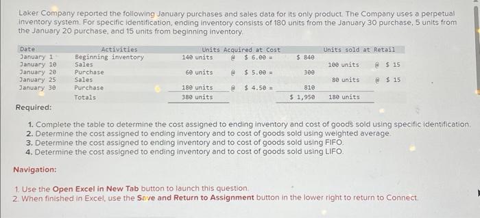
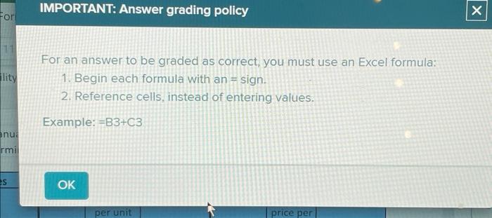
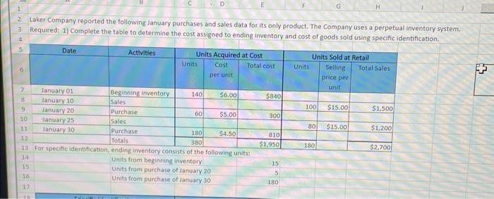
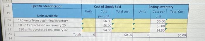
For an answer to be graded as correct, you must use an Excel formula: 1. Begin each formula with an = sign. 2. Reference cells, instead of entering values. Example: =B3+C3 Laker Company reported the following January purchases and sales data for its only product. The Company uses a perpetual inventory system. Required: 1) Complete the table to determine the cost assigned to ending inventory and cost of goods sold using specific identification. Laker Company reported the following January purchases and sales data for its only product. The Company uses a perpetual inventory system. For specific identification, ending inventory consists of 180 units from the January 30 purchase, 5 units from the January 20 purchase, and 15 units from beginning inventory. 1. Complete the table to determine the cost assigned to ending inventory and cost of goods sold using specific identification. 2. Determine the cost assigned to ending inventory and to cost of goods sold using weighted average. 3. Determine the cost assigned to ending inventory and to cost of goods sold using FIFO. 4. Determine the cost assigned to ending inventory and to cost of goods sold using LIFO. Navigation: 1. Use the Open Excel in New Tab button to launch this question. 2. When finished in Excel, use the Sive and Return to Assignment button in the lower right to return to Connect. \begin{tabular}{|c|c|c|c|c|c|c|c|} \hline 18 & Specific Identification & & Dst of Goods & Sold & & nding Invent & ory \\ \hline 19 & Units available & Units & Costperunit & Total cost & Units & Costperunit & Total Cost \\ \hline 20 & 140 units from beginning inventory & & $6.00 & & & $6.00 & \\ \hline 21 & 60 units purchased on January 20 & & $5.00 & & & $5.00 & \\ \hline 22 & 180 units purchased on January 30 & & $4.50 & 7 & & $4.507 & \\ \hline 23 & Totals & 0 & & $0.00 & o) & & $0.00 \\ \hline \end{tabular}