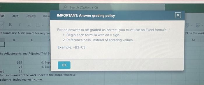
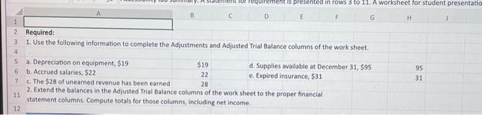
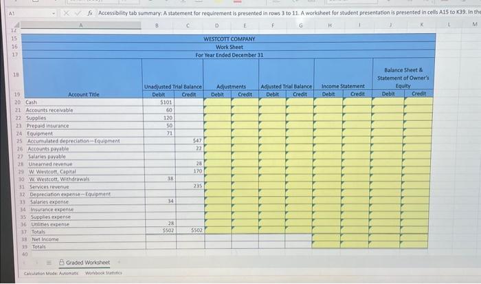
For an answer to be graded as correct, you must use an Excel formula: 1. Begin each formula with an = sign. 2. Reference cells, instead of entering values. Example: =B3+C3 he Adjustments and Adjusted Trial B lance columns of the work sheet to the proper financial columns, Including net income. 1 2 Required: 3 1. Use the following information to complete the Adjustments and Adjusted Trial Balance columns of the work sheet. 4 5 a. Depreciation on equipment, $19 b. Accrued salaries, $22 $19 22 d. Supplies available at December 31, \$95 e. Expired insurance, $31 c. The $28 of unearned revenue has been earned 28 2. Extend the balances in the Adjusted Trial Balance columns of the work sheet to the proper financial statement columns. Compute totals for those columns, including net income. A1 fx Accessibility tab summary. A statement for requirement is presented in rows 3 to 11 . A workheet for student presentation is presented in cells A15 to X39, In the