For expert using R sorry I post this question without data before?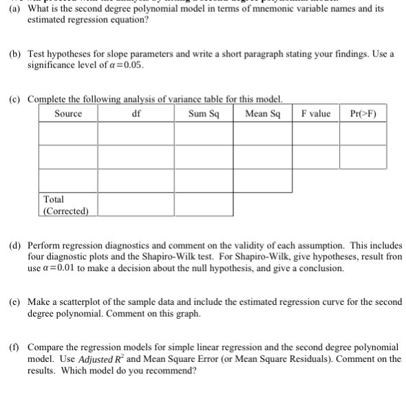

Simple Linear Regression and Polynomial Regression

# HW 2

#

# Read data from csv file

data

head(data)

str(data)

# scatterplot of independent and dependent variables

plot(data$pectin,data$firmness,xlab="Pectin, %",ylab="Firmness")

par(mfrow = c(2, 2)) # Split the plotting panel into a 2 x 2 grid

model

summary(model)

anova(model)

plot(model)

shapiro.test(resid(model))

# examine histogram and boxplot of residuals

par(mfrow = c(1, 1))

hist(resid(model))

boxplot(resid(model))

# predict dependent variable for specified value of independent variable

predict(model, data.frame(pectin = 1.5))

# Estimated regression line and scatterplot of data

plot(data$pectin,data$firmness,xlab="Pectin, %", ylab="Firmness",

ylim=c(45,75),xlim=c(0,3),main="Simple Linear Regression",

pch=19,cex=1.5)

lines(sort(data$pectin),fitted(model)[order(data$pectin)], col="blue", type="l")

par(mfrow = c(2, 2))

# fit a second degree polynomial

# create quadratic term for pectin

data$pectinSq

model2

summary(model2)

anova(model2)

plot(model2)

shapiro.test(resid(model2))

par(mfrow = c(1, 1))

hist(resid(model2))

boxplot(resid(model2))

# predict dependent variable for specified value of independent variable

predict(model2, data.frame(pectin = 1.5, pectinSq=2.25))

# Estimated regression line and scatterplot of data

plot(data$pectin,data$firmness,xlab="Pectin, %", ylab="Firmness",

ylim=c(45,75),xlim=c(0,3),main="Simple Linear Regression",

pch=19,cex=1.5)

lines(sort(data$pectin),fitted(model2)[order(data$pectin)], col="blue", type="l")

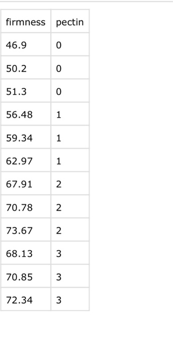
(a) What is the second degree polynomial model in terms of mnemonic variable names and its estimated regression equation? (b) Test hypotheses for slope parameters and write a short paragraph stating your findings. Use a significance level of -0.05. (c) Complete the following analysis of variance table for this model. Source df Sum SqMean S F valuePrF) Total Corrected) (d) Perform regression diagnostics and comment on the validity of each assumption. This includes four diagnostic plots and the Shapiro-Wilk test. For Shapiro-Wilk, give hypotheses, result fron use a-0.01 to make a decision about the null hypothesis, and give a conclusion. (e) Make a scatterplot of the sample data and include the estimated regression curve for the second degree polynomial. Comment on this graph. () Compare the regression models for simple linear regression and the second degree polynomial model. Use Adjusted R and Mean Square Error (or Mean Square Residuals). Comment on the results. Which model do you recommend? firmness pectin 46.9 50.2 51.3 56.48 1 59.34 1 62.97 1 67.912 70.78 2 73.672 68.13 70.85 3 72.34 3 0 0