Forecasting Case Analysis

MGT 3332

Fall 2019

The Fresh Detergent Case

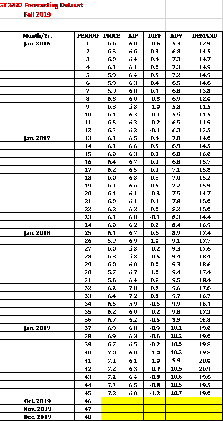
Enterprise Industries produces Fresh, a brand of liquid detergent. In order to more effectively manage its inventory, the company would like to better predict demand for Fresh. To develop a prediction model, the company has gathered data concerning demand for Fresh over the last 45 sales periods. Each sales period is defined as one month. The variables are as follows:

Demand = Y = demand for a large size bottle of Fresh (in 100,000)

Price = the price of Fresh as offered by Ent. Industries

AIP = the average industry price

ADV = Ent. Industries Advertising Expenditure (in $100,000) to Promote Fresh in the sales period.

DIFF = AIP - Price = the "price difference" in the sales period

1- Download the data from Course Blackboard site into Excel spreadsheet.

2- Make time series scatter plots of all five variables (five graphs). Insert trend line, equation, and R-squared. Observe graphs and provide interpretation of results.

3- Construct scatter plots of Demand vs. DIFF and Demand vs. ADV, Demand vs. AIP, and Demand vs. Price. Insert fitted line, equation, and R-squared. Observe graphs and provide interpretation. Note that Demand is always on the Y axis.

4- Obtain the correlation matrix for all six variables and list the variables that have strong correlation with Demand. High correlation is r > 0.50. Explain your findings in plain language.

5- Use 3-month and 6-month moving averages to predict the demand for October 2019. Find MAD for both forecasts and identify the preferred one based on each calculation. Is the moving average suitable method for forecasting for this data set? Explain your reasoning.

6- Use weighted moving averages if weights of 1, 2, ..., 45 (are used periods as weights for each month) to predict October 2019 demand. Explain your reasoning.

7- Use Exponential smoothing forecasts with alpha of 0.1, 0.2, ..., 0.9 to predict October 2019 demand. Identify the value of alpha that results in the lowest MAD.

8- Find the monthly seasonal indices for the demand values using Simple Average (SA) method. Find the de-seasonalized demand values by dividing monthly demand by seasonal indices.

9- Use regression to perform trend analysis on the de-seasonalized demand values. Is trend analysis suitable for this data? Find MAD and explain the Excel Regression output (trend equation, r, r-squared, goodness of model).

10- Find the seasonally adjusted trend forecasts for October through December 2019.

11- Perform simple linear regression analysis with ADV as the independent variable to predict demand. Write the complete equation, find MAD and explain the Excel Regression output. Make sure to use the de-seasonalized demand data for this model and all future models.

12- Repeat part (11) with DIFF as the independent variable.

13- Construct multiple linear regression model with Period, AIP, DIFF, and ADV as independent variables. Formulate the equation, find MAD, and explain the output. Rank variables based on their degree of contribution to the model. Observe significant F, R-squared, and p-values and explain.

14- Perform multiple linear regression analysis with Period, DIFF, and ADV as independent variables. Formulate the equation and find MAD. Which variable is the most significant predictor of demand? Rank the independent variables based on their degree of contribution to the model. Observe significant F, R-squared, and p-values and explain.

15- Use the model obtained in parts 14 and make forecasts for the following months. Make sure to seasonalize final forecasts.

Period Price AIP ADV

Oct. 2019 $3.30 $9.65 $11.7

Nov. 2019 $3.45 $9.70 $11.8

Dec. 2019 $3.80 $9.95 $12.1

16- Provide a case conclusion based on above analysis.

NOTE: I NEED TO SEE THE EXCEL PROCESS IN EACH QUESTION , PLEASE ATTACHMENT THE WORK EXCEL. submit a copy of Word file and Excel file of their work Please...!!!

ST 3332 Forecasting Dataset Fall 2019 Month/Yr. Jan. 2016 Jan. 2017 21 PERIOD PRICE AIP 6.6 6.0 2 6.3 16. 6 6.0 6.4 6.1 6.1 5.9 6.4 5.9 6.3 5.9 6.0 6.8 6.0 6.8 5.8 10 6.4 16.3 11 6.5 6.3 12 6.3 6.2 13 6.1 6.5 14 6.1 6.6 15 6.0 6.3 16 6.4 6.7 17 16.2 6.5 18 6.0 6.8 19 6 .1 6.6 20 6.4 6.1 6.0 6.1 22 6.2 6.2 23 6.1 6.0 24 6.0 6.2 25 6.1 6.7 26 5.9 6.9 27 6.0 5.8 28 6.3 5.8 29 6.0 6.0 5.7 6.7 31 5.6 6.4 32 6.2 7.0 33 6.4 7.2 34 6.5 1 5 .9 35 6.2 6.0 36 6.7 6.2 37 6.9 6.0 38 16.9 6.3 39 16.7 6.5 40 7.0 6.0 41 7.1 6.1 42 7.2 6.3 43 7.2 6.4 7.3 6.5 45 7.2 6.0 DIFF | ADV -0.6 5.3 0 .3 6.8 0.4 7.3 0.0 7.3 0.5 l 7.2 10.4 6.5 6.1 6.8 -0.8 16.9 -1.0 5.8 -0.1 5.5 -0.2 6.5 -0.1 6.3 0.4 7.0 0.5 6.9 0.3 6.8 0.3 6.8 0.3 7.1 0.8 7.0 0.5 l 7.2 -0.3 7.5 0.1 7.8 0. 0 8 .2 -0.1 8.3 0.2 8.4 0.6 8.9 1.0 9.1 -0.2 9.3 -0.5 9.4 0.0 9.3 1.0 9.4 0.8 9.5 0.8 9.6 0.8 9.7 -0.6 9.9 -0. 2 9 .8 -0.5 9.9 -0.9 10.1 -0.6 10.2 -0.2 10.5 -1.0 10.3 -1.0 9.9 -0.9 10.5 -0.8 10.6 -0.8 10.5 -1.2 10.7 DEMAND 12.9 14.5 14.7 14.9 14.9 14.6 13.8 12.0 11.5 11.5 11.9 13.5 14.0 14.5 16.0 15.7 15.8 15.2 15.9 14.7 15.0 15.0 14.4 16.9 17.4 17.7 17.6 18.4 18.6 17.4 18.4 17.6 16.7 16.1 17.3 16.8 19.0 19.0 19.8 19.8 20.0 20.9 19.6 19.5 19.0 Jan. 2018 Jan. 2019 44 46 Oct 2019 Nov. 2019 Dec. 2019 47 48 ST 3332 Forecasting Dataset Fall 2019 Month/Yr. Jan. 2016 Jan. 2017 21 PERIOD PRICE AIP 6.6 6.0 2 6.3 16. 6 6.0 6.4 6.1 6.1 5.9 6.4 5.9 6.3 5.9 6.0 6.8 6.0 6.8 5.8 10 6.4 16.3 11 6.5 6.3 12 6.3 6.2 13 6.1 6.5 14 6.1 6.6 15 6.0 6.3 16 6.4 6.7 17 16.2 6.5 18 6.0 6.8 19 6 .1 6.6 20 6.4 6.1 6.0 6.1 22 6.2 6.2 23 6.1 6.0 24 6.0 6.2 25 6.1 6.7 26 5.9 6.9 27 6.0 5.8 28 6.3 5.8 29 6.0 6.0 5.7 6.7 31 5.6 6.4 32 6.2 7.0 33 6.4 7.2 34 6.5 1 5 .9 35 6.2 6.0 36 6.7 6.2 37 6.9 6.0 38 16.9 6.3 39 16.7 6.5 40 7.0 6.0 41 7.1 6.1 42 7.2 6.3 43 7.2 6.4 7.3 6.5 45 7.2 6.0 DIFF | ADV -0.6 5.3 0 .3 6.8 0.4 7.3 0.0 7.3 0.5 l 7.2 10.4 6.5 6.1 6.8 -0.8 16.9 -1.0 5.8 -0.1 5.5 -0.2 6.5 -0.1 6.3 0.4 7.0 0.5 6.9 0.3 6.8 0.3 6.8 0.3 7.1 0.8 7.0 0.5 l 7.2 -0.3 7.5 0.1 7.8 0. 0 8 .2 -0.1 8.3 0.2 8.4 0.6 8.9 1.0 9.1 -0.2 9.3 -0.5 9.4 0.0 9.3 1.0 9.4 0.8 9.5 0.8 9.6 0.8 9.7 -0.6 9.9 -0. 2 9 .8 -0.5 9.9 -0.9 10.1 -0.6 10.2 -0.2 10.5 -1.0 10.3 -1.0 9.9 -0.9 10.5 -0.8 10.6 -0.8 10.5 -1.2 10.7 DEMAND 12.9 14.5 14.7 14.9 14.9 14.6 13.8 12.0 11.5 11.5 11.9 13.5 14.0 14.5 16.0 15.7 15.8 15.2 15.9 14.7 15.0 15.0 14.4 16.9 17.4 17.7 17.6 18.4 18.6 17.4 18.4 17.6 16.7 16.1 17.3 16.8 19.0 19.0 19.8 19.8 20.0 20.9 19.6 19.5 19.0 Jan. 2018 Jan. 2019 44 46 Oct 2019 Nov. 2019 Dec. 2019 47 48